Plot Ceteris Paribus Explanations
Function 'plot.ceteris_paribus_explainer' plots Ceteris Paribus Plots for selected observations. Various parameters help to decide what should be plotted, profiles, aggregated profiles, points or rugs.
# S3 method for ceteris_paribus_explainer
plot(x, ..., size = 1, alpha = 0.3,
  color = "black", size_points = 2, alpha_points = 1,
  color_points = color, size_rugs = 0.5, alpha_rugs = 1,
  color_rugs = color, size_residuals = 1, alpha_residuals = 1,
  color_residuals = color, only_numerical = TRUE,
  show_profiles = TRUE, show_observations = TRUE, show_rugs = FALSE,
  show_residuals = FALSE, aggregate_profiles = NULL, as.gg = FALSE,
  facet_ncol = NULL, selected_variables = NULL)
Arguments
| x | a ceteris paribus explainer produced with function `ceteris_paribus()` |
|---|---|
| ... | other explainers that shall be plotted together |
| size | a numeric. Size of lines to be plotted |
| alpha | a numeric between 0 and 1. Opacity of lines |
| color | a character. Either name of a color or name of a variable that should be used for coloring |
| size_points | a numeric. Size of points to be plotted |
| alpha_points | a numeric between 0 and 1. Opacity of points |
| color_points | a character. Either name of a color or name of a variable that should be used for coloring |
| size_rugs | a numeric. Size of rugs to be plotted |
| alpha_rugs | a numeric between 0 and 1. Opacity of rugs |
| color_rugs | a character. Either name of a color or name of a variable that should be used for coloring |
| size_residuals | a numeric. Size of line and points to be plotted for residuals |
| alpha_residuals | a numeric between 0 and 1. Opacity of points and lines for residuals |
| color_residuals | a character. Either name of a color or name of a variable that should be used for coloring for residuals |
| only_numerical | a logical. If TRUE then only numerical variables will be plotted. If FALSE then only categorical variables will be plotted. |
| show_profiles | a logical. If TRUE then profiles will be plotted. Either individual or aggregate (see `aggregate_profiles`) |
| show_observations | a logical. If TRUE then individual observations will be marked as points |
| show_rugs | a logical. If TRUE then individual observations will be marked as rugs |
| show_residuals | a logical. If TRUE then residuals will be plotted as a line ended with a point |
| aggregate_profiles | function. If NULL (default) then individual profiles will be plotted. If a function (e.g. mean or median) then profiles will be aggregated and only the aggregate profile will be plotted |
| as.gg | if TRUE then returning plot will have gg class |
| facet_ncol | number of columns for the `facet_wrap()` |
| selected_variables | if not NULL then only `selected_variables` will be presented |
Value
a ggplot2 object
Examples
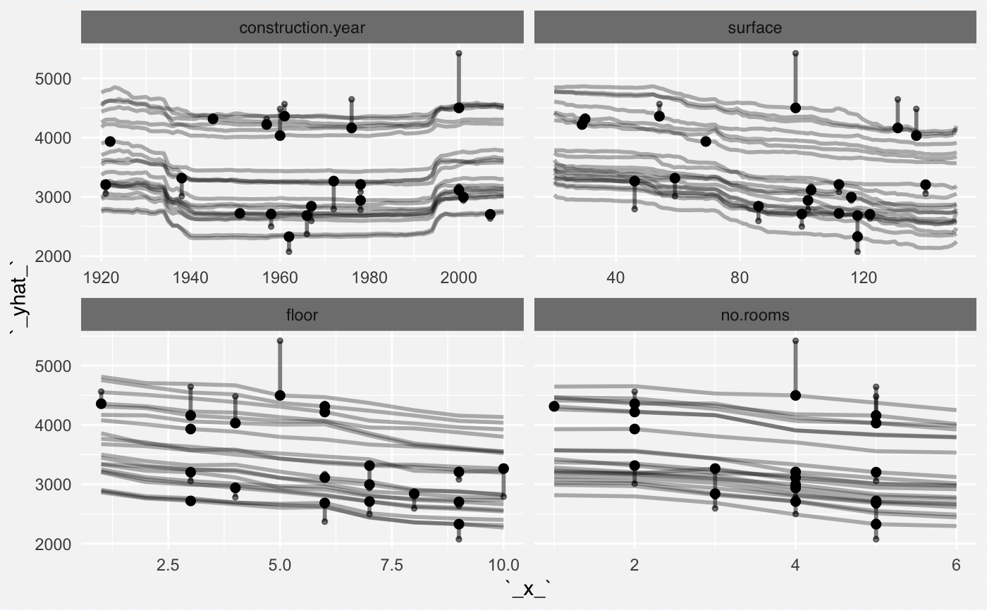
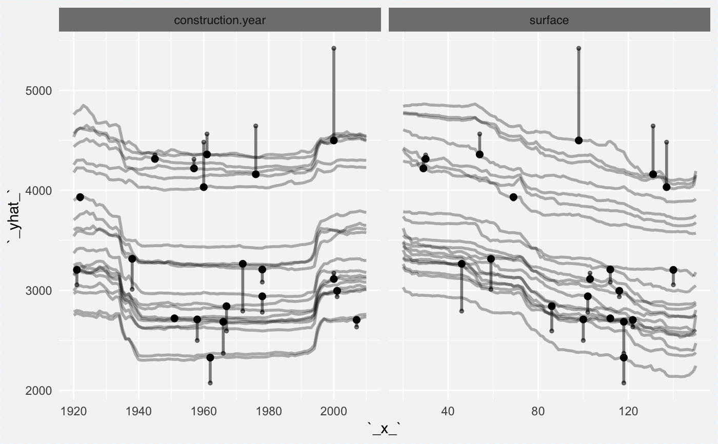
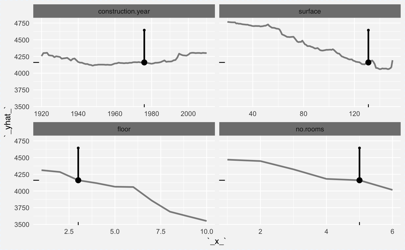
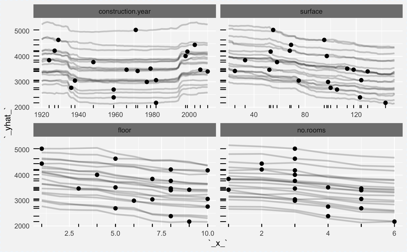
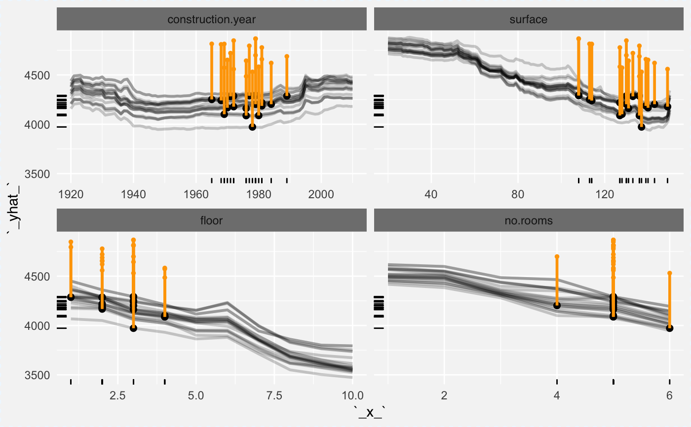
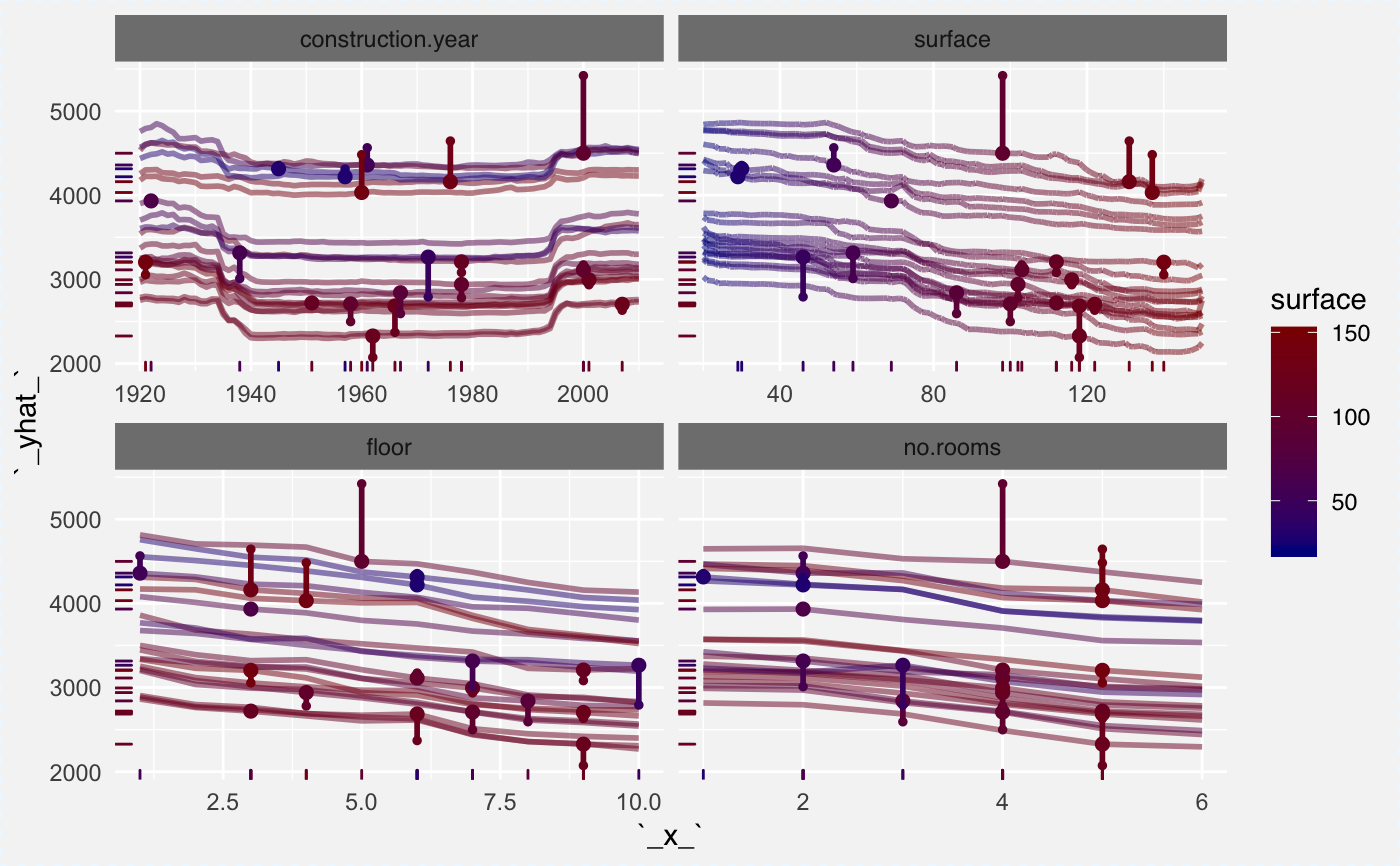
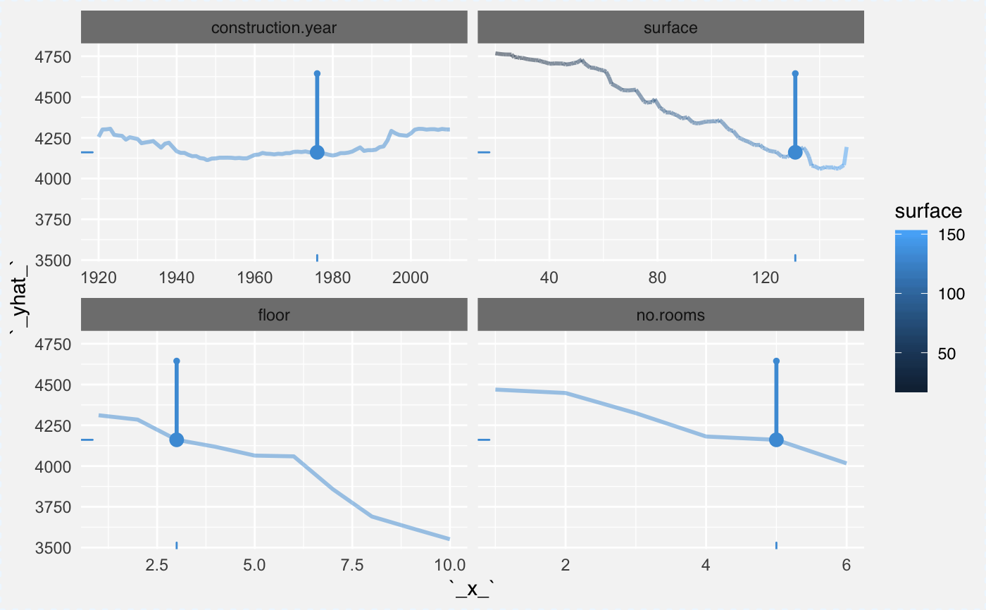
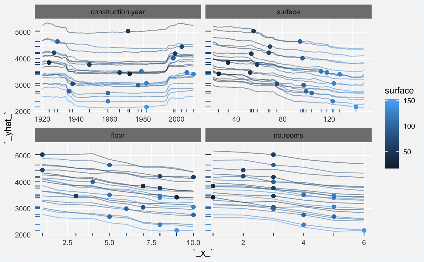
library("DALEX")library("randomForest") set.seed(59) apartments_rf_model <- randomForest(m2.price ~ construction.year + surface + floor + no.rooms + district, data = apartments) explainer_rf <- explain(apartments_rf_model, data = apartmentsTest[,2:6], y = apartmentsTest$m2.price) apartments_small <- apartmentsTest[1:20,] apartments_small_1 <- apartmentsTest[1,] apartments_small_2 <- select_sample(apartmentsTest, n = 20) apartments_small_3 <- select_neighbours(apartmentsTest, apartments_small_1, n = 20) cp_rf <- ceteris_paribus(explainer_rf, apartments_small) cp_rf_1 <- ceteris_paribus(explainer_rf, apartments_small_1) cp_rf_2 <- ceteris_paribus(explainer_rf, apartments_small_2) cp_rf_3 <- ceteris_paribus(explainer_rf, apartments_small_3) cp_rf#> Top profiles : #> m2.price construction.year surface floor no.rooms district _yhat_ #> 1001 4644 1920 131 3 5 Srodmiescie 4255.354 #> 1001.1 4644 1921 131 3 5 Srodmiescie 4300.702 #> 1001.2 4644 1922 131 3 5 Srodmiescie 4301.926 #> 1001.3 4644 1923 131 3 5 Srodmiescie 4305.352 #> 1001.4 4644 1923 131 3 5 Srodmiescie 4305.352 #> 1001.5 4644 1924 131 3 5 Srodmiescie 4267.723 #> _vname_ _ids_ _label_ #> 1001 construction.year 1001 randomForest #> 1001.1 construction.year 1001 randomForest #> 1001.2 construction.year 1001 randomForest #> 1001.3 construction.year 1001 randomForest #> 1001.4 construction.year 1001 randomForest #> 1001.5 construction.year 1001 randomForest #> #> #> Top observations: #> m2.price construction.year surface floor no.rooms district _yhat_ #> 1001 4644 1976 131 3 5 Srodmiescie 4160.840 #> 1002 3082 1978 112 9 4 Mokotow 3208.201 #> 1003 2498 1958 100 7 4 Bielany 2708.745 #> 1004 2735 1951 112 3 5 Wola 2719.604 #> 1005 2781 1978 102 4 4 Bemowo 2939.989 #> 1006 2936 2001 116 7 4 Bemowo 2995.042 #> _label_ #> 1001 randomForest #> 1002 randomForest #> 1003 randomForest #> 1004 randomForest #> 1005 randomForest #> 1006 randomForestcp_rf_y <- ceteris_paribus(explainer_rf, apartments_small, y = apartments_small$m2.price) cp_rf_y1 <- ceteris_paribus(explainer_rf, apartments_small_1, y = apartments_small_1$m2.price) cp_rf_y2 <- ceteris_paribus(explainer_rf, apartments_small_2, y = apartments_small_2$m2.price) cp_rf_y3 <- ceteris_paribus(explainer_rf, apartments_small_3, y = apartments_small_3$m2.price) plot(cp_rf_y, show_profiles = TRUE, show_observations = TRUE, show_residuals = TRUE, color = "black", alpha = 0.3, alpha_points = 1, alpha_residuals = 0.5, size_points = 2, size_rugs = 0.5)plot(cp_rf_y, show_profiles = TRUE, show_observations = TRUE, show_residuals = TRUE, color = "black", selected_variables = c("construction.year", "surface"), alpha = 0.3, alpha_points = 1, alpha_residuals = 0.5, size_points = 2, size_rugs = 0.5)plot(cp_rf_y1, show_profiles = TRUE, show_observations = TRUE, show_rugs = TRUE, show_residuals = TRUE, alpha = 0.5, size_points = 3, alpha_points = 1, size_rugs = 0.5)plot(cp_rf_y2, show_profiles = TRUE, show_observations = TRUE, show_rugs = TRUE, alpha = 0.2, alpha_points = 1, size_rugs = 0.5)plot(cp_rf_y3, show_profiles = TRUE, show_rugs = TRUE, show_residuals = TRUE, alpha = 0.2, color_residuals = "orange", size_rugs = 0.5)plot(cp_rf_y, show_profiles = TRUE, show_observations = TRUE, show_rugs = TRUE, size_rugs = 0.5, show_residuals = TRUE, alpha = 0.5, color = "surface", as.gg = TRUE) + scale_color_gradient(low = "darkblue", high = "darkred")plot(cp_rf_y1, show_profiles = TRUE, show_observations = TRUE, show_rugs = TRUE, show_residuals = TRUE, alpha = 0.5, color = "surface", size_points = 3)plot(cp_rf_y2, show_profiles = TRUE, show_observations = TRUE, show_rugs = TRUE, size = 0.5, alpha = 0.5, color = "surface")plot(cp_rf_y, show_profiles = TRUE, show_rugs = TRUE, size_rugs = 0.5, show_residuals = FALSE, aggregate_profiles = mean, color = "darkblue")