Model Agnostic Experimental Approach to Break Down Plots with Interactions

This function implements decomposition of model predictions with identification of interactions. The complexity of this function is O(2*p) for additive models and O(2*p^2) for interactions. This function works in similar way to step-up and step-down greedy approaximations, the main difference is that in the fisrt step the order of variables is determied. And in the second step the impact is calculated.

break_down(explainer, new_observation, check_interactions = TRUE,
  keep_distributions = FALSE)

Arguments

explainer	a model to be explained, preprocessed by function `DALEX::explain()`.
new_observation	a new observation with columns that corresponds to variables used in the model
check_interactions	the orgin/baseline for the `breakDown`` plots, where the rectangles start. It may be a number or a character "Intercept". In the latter case the orgin will be set to model intercept.
keep_distributions	if TRUE, then the distribution of partial predictions is stored in addition to the average.

Value

an object of the broken class

Examples

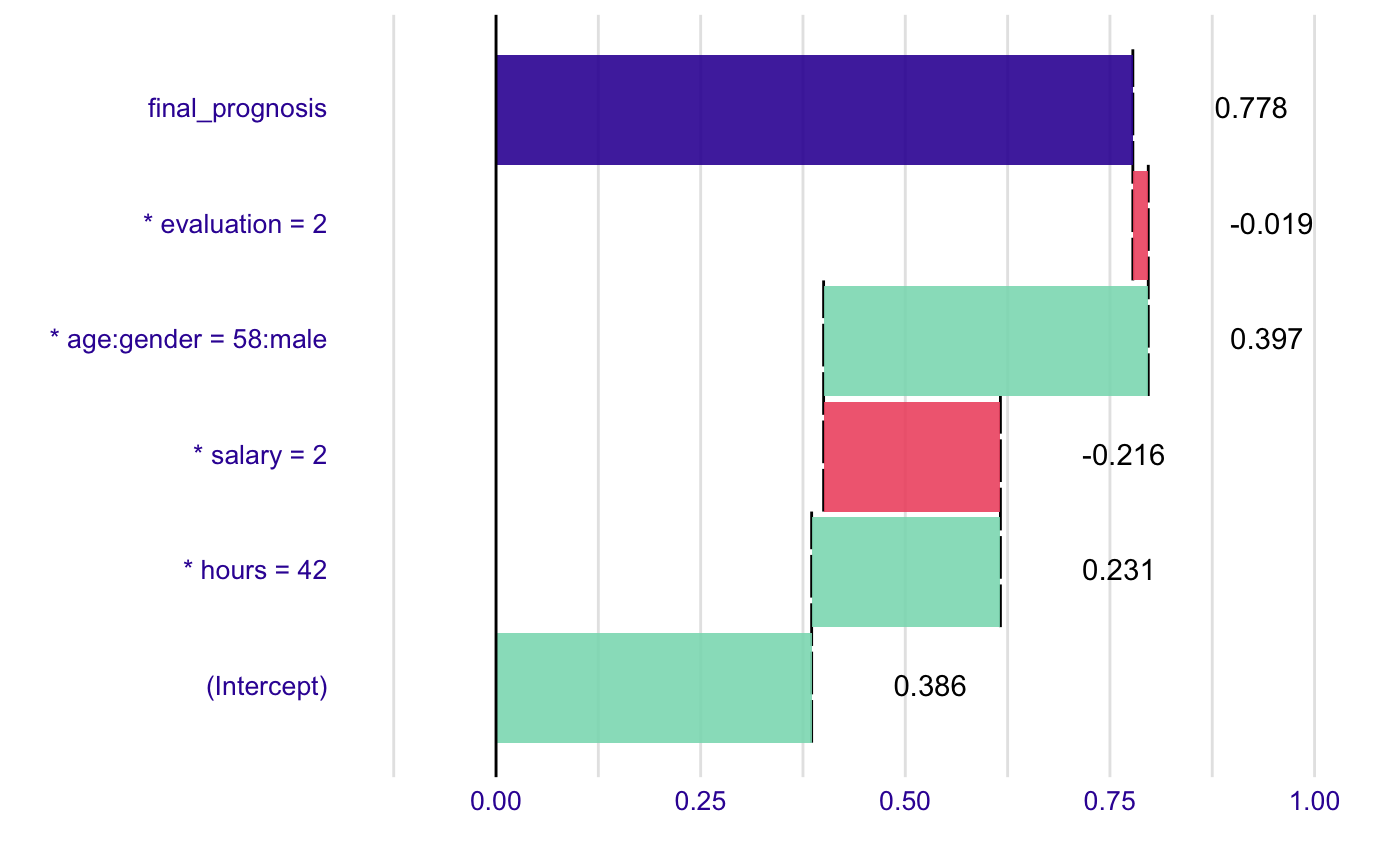
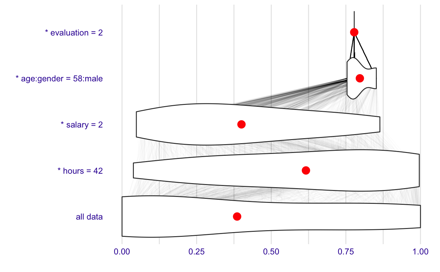
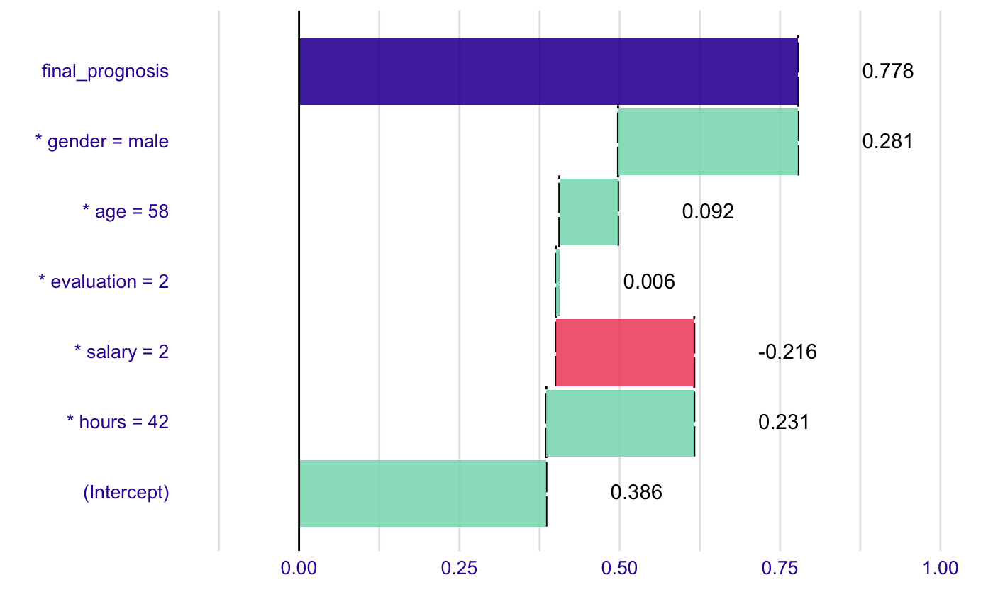
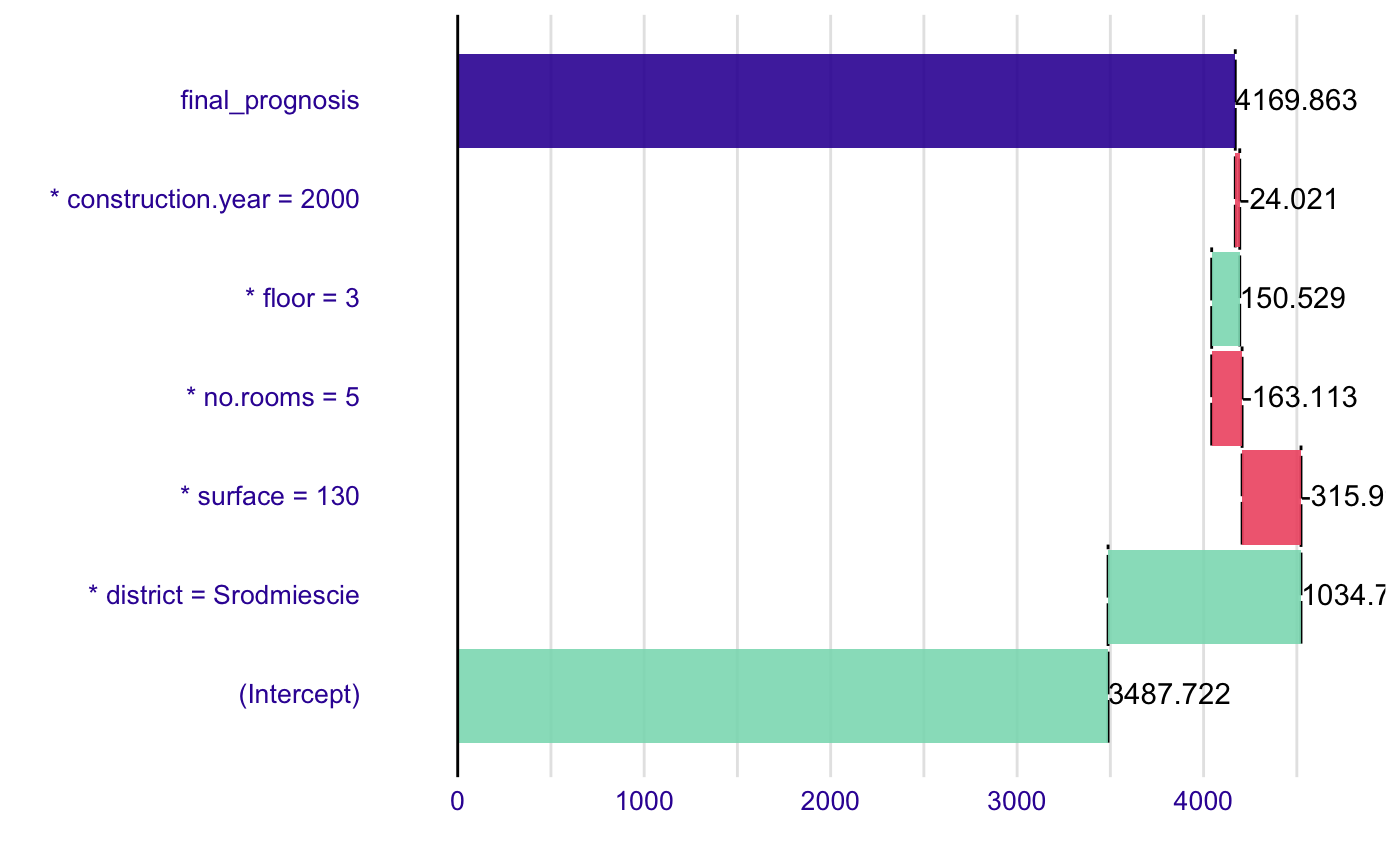
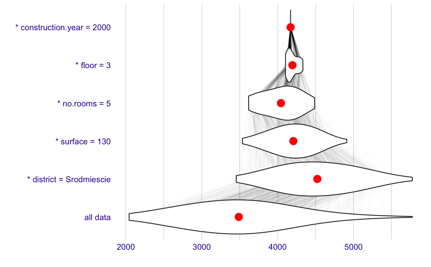
library("DALEX")
library("breakDown")
library("randomForest")
set.seed(1313)
# example with interaction
# classification for HR data
model <- randomForest(status ~ . , data = HR)
new_observation <- HRTest[1,]
data <- HR[1:1000,]
predict.function <- function(m,x) predict(m,x, type = "prob")[,1]

explainer_rf_fired <- explain(model,
                 data = HR[1:1000,1:5],
                 y = HR$status[1:1000] == "fired",
                 predict_function = function(m,x) predict(m,x, type = "prob")[,1],
                 label = "fired")

bd_rf <- break_down(explainer_rf_fired,
                 new_observation,
                 keep_distributions = TRUE)

bd_rf
#>                        contribution
#> (Intercept)                   0.386
#> * hours = 42                  0.231
#> * salary = 2                 -0.216
#> * age:gender = 58:male        0.397
#> * evaluation = 2             -0.019
#> final_prognosis               0.778
#> baseline:  0 
plot(bd_rf)
plot(bd_rf, plot_distributions = TRUE)

bd_rf <- break_down(explainer_rf_fired,
                 new_observation,
                 check_interactions = FALSE,
                 keep_distributions = TRUE)

bd_rf
#>                  contribution
#> (Intercept)             0.386
#> * hours = 42            0.231
#> * salary = 2           -0.216
#> * evaluation = 2        0.006
#> * age = 58              0.092
#> * gender = male         0.281
#> final_prognosis         0.778
#> baseline:  0 
plot(bd_rf)

# example for regression - apartment prices
# here we do not have intreactions
model <- randomForest(m2.price ~ . , data = apartments)
explainer_rf <- explain(model,
         data = apartmentsTest[1:1000,2:6],
         y = apartmentsTest$m2.price[1:1000],
         label = "rf")

bd_rf <- break_down(explainer_rf,
         apartmentsTest[1,],
         check_interactions = FALSE,
         keep_distributions = TRUE)

bd_rf
#>                            contribution
#> (Intercept)                    3487.722
#> * district = Srodmiescie       1034.737
#> * surface = 130                -315.991
#> * no.rooms = 5                 -163.113
#> * floor = 3                     150.529
#> * construction.year = 2000      -24.021
#> final_prognosis                4169.863
#> baseline:  0 
plot(bd_rf)
plot(bd_rf, plot_distributions = TRUE)