Chapter 8 Story Lungs: eXplainable predictions for post operational risks

Authors: Maciej Bartczak (UW), Marika Partyka (PW)

Mentors: Aleksandra Radziwiłł (McKinsey & Company), Maciej Krasowski (McKinsey & Company)

8.1 Introduction

Science allows us to understand the world better. New technologies, data collection solves the problems not only of large companies but also of ordinary people. Especially if human life is at stake. They say that cancer is the killer of the 21st century. That’s why even small attempts to subdue this problem are important. In our work, we deal with lung cancer. We try to analise the chances of survival of a patient who has had a tumor removal surgery by explaining predicitve models. Note that we do not generally anticipate the chances of survival here, but only consider a particular group of patients who have cancer and have been qualified for surgery. Therefore, along the way we may encounter many non-intuitive conclusions, we may encounter here the survivorship bias. That is why the role of explaining the model in this case is so important, as we will show in the next parts of this chapter. But let’s focus on the data for a moment.

8.2 Data set

The data set consists of the following varaibles.

Numerical

Variable	Unit
`date_birth`	date
`date_start_treatment`	date
`date_surgery`	date
`tumor_size_x`	cm
`tumor_size_y`	cm
`tumor_size_z`	cm
`years_smoking`	years
`age`	years
`time_to_surgery`	years (“today” - date_surgery)

Categorical

Variable	Decription	Values
`sex`	subject sex	male/female
`histopatological_diagnosis`	type of cancer	Rak płaskonabłonkowy, pleomorficzny, …*
`symptoms`	whether symptoms were observed	yes/no
`lung_cancer_in_family`	whether family member had cancer	yes/no
`stadium_uicc`	severity of tumor	IA1, IA2, IA3, IB, IIA, IIB, IIIA, IIIB, IVA, IVB*
`alive`	whether subject is alive	yes/no (the target variable)

About 1/3 af values of varaibles annotated with * was missing.

Survivability was registered in a certain point of time - December 2016. That’s why we transform all the date varriables to number of years to December 2016. There are two reasons: - by changing dates to ages, i.e. date_surgery to age_when_surgery_was_performed we wouldn’t capture the time between the surgery and “today”. The longer it is the “more time patient has to die”, - similar analysis could be easily performed for different value of “today”.

Following encoding strategy was employed: - binary variables were encoded as 0s and 1s, - categorical variable histopatological_diagnosis was one-hot encoded, - categorical variable stadium_uicc was encoded by increasing integers as there is natural order to this variable.

8.3 Models

We have tried out several models as well as different preprocessing strategies. However, no model yielded better results than scikit-learn’s logistic regression with hyperparameters cross validation.

In order to further refine our model we tried adding some features as well as pruning irrelevent ones. We have added following variables: - tumor_volume = tumor_size_x * tumor_size_y * tumor_size_z, - log_tumor_volume = log(tumor_volume + 1e-4)

and considered two, equally well performing, versions of the data set: - full - with added tumor_volume and log_tumor_volume - pruned - with no histopatological_diagnosis and only log_tumor_volume with regard to the tumor

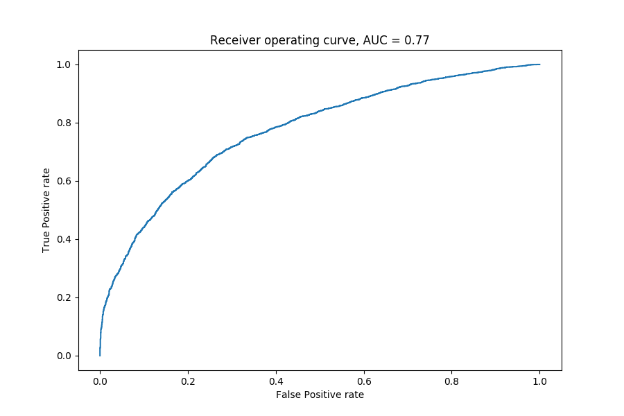
This is the receiver operating curve for the final model.

FIGURE 8.1: ROC for final model.

8.4 Explanations

The explanations are based on logistic regression model.

We base our analysis on 3 methods of explaining models, mainly Ceteris Paribus as well as Shap and Variable Importance. Let’s start by explaining at the dataset level. Let’s see how Variable Importance behaves.

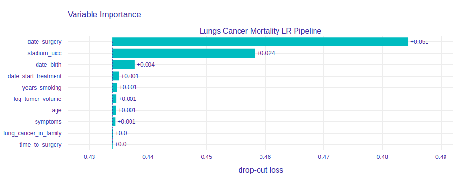
Variable Importance for Logistic Regression model. Under the date_surgery variable is the number of years that have elapsed between that date and the end of the study. As the explanation shows that this variable is the most important, we will look at it in more detail later in this chapter.

FIGURE 8.2: Variable Importance for Logistic Regression model. Under the date_surgery variable is the number of years that have elapsed between that date and the end of the study. As the explanation shows that this variable is the most important, we will look at it in more detail later in this chapter.

The second most important is the UICC stage. This variable tells us how advanced the cancer we cut out is. You can guess that the more advanced the stage, the bigger and harder the tumor is to cut out. We may wonder why the third most important variable is date of birth, not age. In fact, these two variables are obviously very correlated and the above results are the result of the distribution of importance between the two variables. Interestingly, the period of time the patient smoked cigarettes does not affect the outcome too much. Of course, if we were to consider the chances of getting lung cancer, or overall survival, this variable could be much more important. However, let’s remember that our study involves patients who are already in advanced disease and undergoing surgery anyway, so how many years they have smoked doesn’t have to be so important at this point.

After a general look at the significance of variables, it is time to go into details. It would be useful if we could explain to the patient why his chances of survival after surgery are as high as our model predicted and show him what would increase or decrease his chances.

For example, let’s take a patient with the following variable values: - date_start_treatment 4.4 - sex K - years_smoking 0 - lung_cancer_in_family No - symptoms No - stadium_uicc IIIB - age 72 - time_to_surgery 0 - log_tumor_volume 5.8 Our most recent model indicated that the chances of survival after surgery for such a patient are \(43\%.\) Here we have an explanation of this result by SHAP.

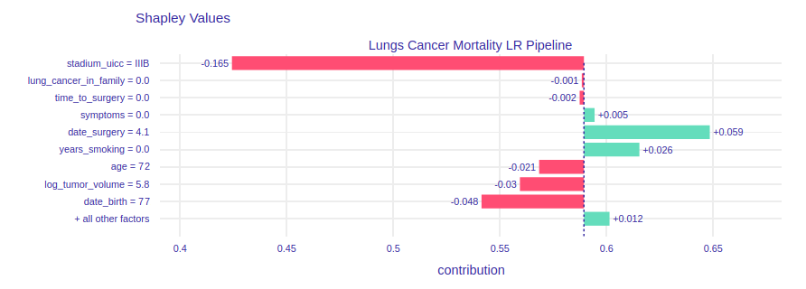
FIGURE 8.3: Shap method for choosen patient.

We see that, according to the conclusions of the previous method, variables stadium_uicc and date_surgery have the greatest impact. The SHAP method allows us to see whether individual variables have a negative or rather positive impact on predictions. Our patient’s stadium_uicc is quite advanced, so it reduces the chances of survival after surgery quite drastically. The date_surgery variable, on the other hand, increases the probability, but we do not know whether a smaller value could further improve our prediction or the opposite.

To find out, we use another Ceteris Paribus method. First we’ll look at the date variables. If we look at the age variable, i.e. the age at the time of surgery, we can see that it behaves quite intuitively. The younger the patient, the better he is able to recover from surgery, so his chances for survival are higher.

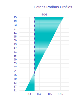
FIGURE 8.4: Ceteris Paribus for age variable.

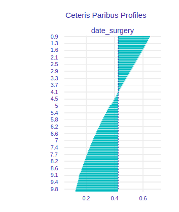
The date_surgery variable is interesting. It indicates the number of years that have passed from surgery to the end of the study. It would seem that the earlier we do surgery, the better our prognosis will be. The charts show the opposite. This may be because if the surgery was done a long time ago, the patient has been getting older since then and has little chance of survival.

FIGURE 8.5: Ceteris Paribus for date_surgery variable.

Now let’s look at the stadium. As mentioned earlier, the more advanced the stage of cancer the worse for the patient. Our patient’s stadium is quite advanced, which has a big influence on the predictions, but if she had a more benign stage her chances of survival would increase strongly.

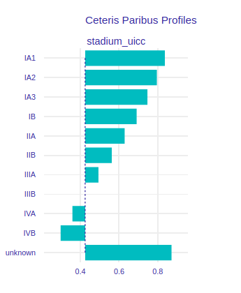
FIGURE 8.6: Ceteris Paribus for stadium_uicc variable.

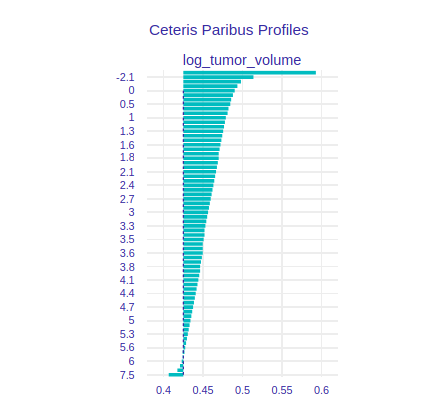
The variable log_tumor_volume indicates that if we cut out a smaller tumor, our postoperative survival increases. This conclusion coincides with our intuition, the removal of a smaller tumor is much safer, because perhaps with a larger one we could damage certain structures and thus increase mortality.

FIGURE 8.7: Ceteris Paribus for the volume of the tumor, but after transformation as a logarithm.

Using model explanations not only helps to explain the result of the prediction, it can also give a hint how to improve our model.

When we built the model on all variables, the explanations allowed us to find highly dependent variables. Let’s compare the CeterisParibus results for the full model and the pruned one. The image below shows the date_birth variable in its original version, i.e. as date.

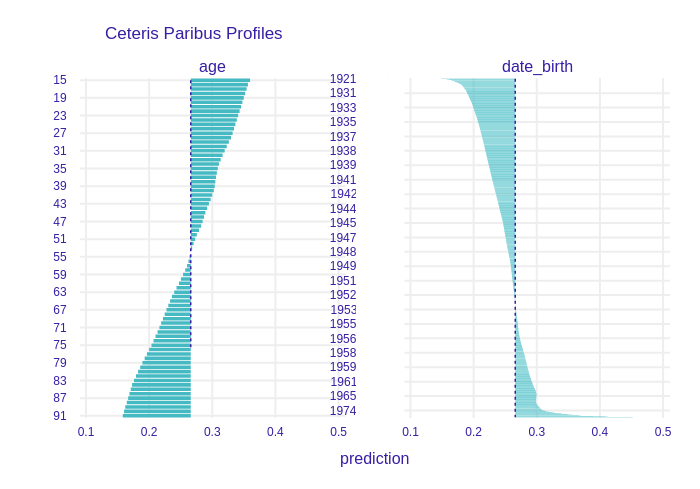
FIGURE 8.8: Selected model with correlated variables left.

In the picture above you can see that the influence of two correlated variables was distributed between them, but after leaving only one of these variables, the influence accumulated on it (picture below).

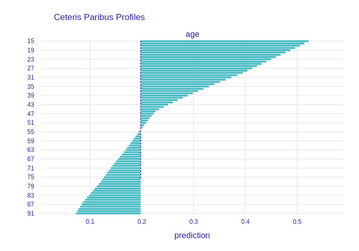
FIGURE 8.9: Model after removing correlated variables, you can see a big difference in the explanation.

At this stage we can already conclude that the techniques of model explanations are not only useful at the end of our journey. They can give us tips on how to transform data or which variables should be deleted.

8.5 Summary and conclusions

XAI methods legitimised employed approach of pruning the dataset.
XAI methods yielded explainations consistent with biological intuintion, what builds up trust in the model.
As variety of modelling and preprocessing approaches resulted in similar predicitive performance we conclude there is not much more to squeeze out of the dataset.