Chapter 6 Story MEPS: Explainable predictions for healthcare expenditures

Authors: Anna Kozioł (Warsaw University of Technology), Katarzyna Lorenc (Warsaw University of Technology), Piotr Podolski (University of Warsaw)

Mentors: Maciej Andrzejak (McKinsey & Company), Alicja Jośko (McKinsey & Company)

6.1 Introduction

Perhaps the most urgent problem with the current health care system in the United States is its high cost. According to the Centers for Disease Control and Prevention, during 2017 health care spending per capita averaged nearly $11,000 and total spending was $3.2 trillion, or 17.9% of GDP. This raises the natural question of the causality of high expenses and the estimation of them for a particular person.

One of the objectives of this chapter is to forecast annual spending on the health care of individuals in the United States.

There is no doubt that these forecasts are of interest to people directly related to medical expenditure, for example, insurance companies, employers, government.

How to deal with a situation when the model works well but is a so-called black box and we do not know what affects a specific result? What if the proposed models return non-intuitive results and we want to know why they are wrong?

The next and main purpose of this chapter is to address these concerns using Explanatory Model Analysis.
We will try to identify not only which features are most predictable for the results, but also the nature of the relationship (e.g. its direction and shape). We will focus on understanding the behavior of the model as a whole, as well as in a specific instant level (for specific person).

The data set comes from a study called Medical Expenditure Panel Survey (MEPS), which is sponsored by the Healthcare Quality and Research Agency. About 15,000 households are selected as a new panel of surveyed units, regularly since 1996.

Data set used for analysis is available for free on the MEPS website. The MEPS contains a representative sample of the population from the United States with two major components: the Household Component and the Insurance Component.

Household Component collects data about demographic characteristics, health conditions, health status, medical history, fees and sources of payment, access to care, satisfaction with care, health insurance coverage, income, and employment for each person surveyed.

The second component - insurance - collects data about the health insurance from private and public sector employers. The data include the number and types of private insurance schemes offered, premiums, employers’ and employees’ health insurance contributions, benefits associated with these schemes, and employer characteristics.

The data processing and analysis were carried out in Python 3.7.3 and R 3.6.1.

6.2 Model

6.2.1 Data

Agency of Healthcare Research and Quality provides an extensive database of medical expenses. Consequently, dataset selection on which we will make further analysis was an important first step. We decided to choose the two latest panels. Expenditures for treatment that we will examine in the following chapter apply to the years 2015/2016 and 2016/2017. The selected dataset contains information on over 32,000 patients, and each of them is described by 3,700 variables. We attached great importance to choosing features that would be appropriate for the prediction. The most important criterion adopted is that the variable cannot relate to expenditure associated with any treatment. For this purpose, we looked through several hundred of them and selected 387 most suitable.

As a part of the preprocessing, we removed records that were marked as Inapplicable in the expenditure column. The number of people who didn’t incur expenses is 5504, while the number of patients with “inapplicable” is 407, the percentage respectively are 17% and 1%. The following figures show the distribution of the explained variable.

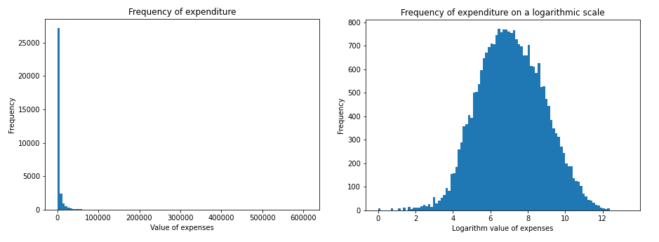
FIGURE 6.1: Distribution of medical expenses

6.3 Model

6.3.1 Data

Agency of Healthcare Research and Quality provides an extensive database of medical expenses. Consequently, data set selection on which we will make further analysis was an important first step. We decided to choose the two latest panels. Expenditures for treatment that we will examine in the following chapter apply to the years 2015/2016 and 2016/2017. The selected dataset contains information on over 32,000 patients, and each of them is described by 3,700 variables. We attached great importance to choosing features that would be appropriate for the prediction. The most important criterion adopted is that the variable cannot relate to expenditure associated with any treatment. For this purpose, we looked through several hundred of them and selected 387 most suitable.

As a part of the preprocessing, we removed records that were marked as Inapplicable in the expenditure column. The number of people with such markings was 407, which is about 1% of the whole data set. The following figures show the distribution of the explained variable.

FIGURE 6.2: Distribution of medical expenses

6.3.2 Model

Among the models we have trained, the best results were achieved by Gradient Boosting. Due to the characteristics of the explained variable, we decided to check the behavior of the model after applying the logarithmic transformation to expenses. In the case of modelling the expenditure logarithm, we also used translations by 1 to avoid undesirable values of the variable. We used NNI toolkit to find the best hyperparameters To choose the best model, we compared the determination coefficient values.

The table below shows the results of the experiments. To calculate the determination coefficient in column \(R^2\) (log), we transformed logarithmically the values of expenses, and after training the model we returned to the original scale.

Values of the determination coefficient.

Model	\(R^2\)	\(R^2\) (log)
Gradient Boosting	0.43	0.44
Tuned Gradient Boosting	0.49	0.46

The best fit relying on the determination coefficient was demonstrated by a Gradient Boosting. Then, as a compromise between the size of the model and its quality, we chose the 7 most important variables. For this purpose, we ranked the significance of the variables in the model and extracted those with the highest coefficient.

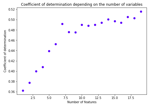
Obtained variables mainly concern the number of visits to specialists. For a more diverse and interesting analysis, we have also taken into account demographic variables such as age, gender, educational background, and race, as well as some disease units.

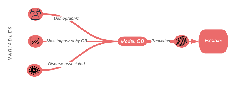
FIGURE 6.3: Scheme of conduct with a specification of origin of variables

A review of selected variables

Variable	New Name	Description
IPNGTDY1	hospital_nights	number of nights associated with hospital discharges
OBDRVY1	phys_visits	number of office-based physician visits
HHAGDY1	home_days	agency home health provider days
DSFTNV5	feet_checked	indicate whether the respondent reported having his or her feet checked for sores or irritations
OBOTHVY1	non-phys_visits	office-based non-physican visits
PSTATS2	disposition	person disposition status
OPOTHVY1	outpatient_visits	outpatient dept non-dr visits
AGE2X	age	age of patient
RACEV2X	race	race of patient
SEX	sex	patient’s gender
HIDEG	edu	the highest degree of education attained at the time the individual entered MEPS
diab_disease	diab_disease	indicates whether the patient suffered from a diabetes disease
art_disease	art_disease	indicates whether the patient suffered from a arthritis disease
ast_disease	ast_disease	indicates whether the patient suffered from a asthma disease
press_disease	press_disease	indicates whether the patient suffered from a high pressure disease
heart_disease	heart_disease	indicates whether the patient suffered from a heart disease

In the following section we will explain the Gradient Boosting model based on 16 variables presented in the table above. The coefficient of determination of the final model is 0.5

6.4 Model Level Explainations

6.4.1 Permutation Variable Importances

In order to find out about the influence of individual variables on the prediction for each patient, we present a Permutation Variable Importances graph.

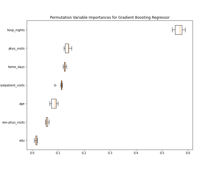
FIGURE 6.4: Permutation Variable Importances for Gradient Boosting Regressor

In the figure 6.4 we present the 6 most relevant variables. Features for which the median of Permutation Variable Importances was less than 0.01 were omitted. Undoubtedly, the most important is the variable that indicates the number of nights spent in the hospital by the patient. An interesting observation seems to us that the demographic variable - age, which initially did not have a significant impact on the prediction, on the reduced model is in the top five most important variables. The remaining demographic variables, as well as those relating to diseases, do not show a gain in relevance in a model reduced to several variables.

6.4.2 Partial Dependence Profiles

Based on previous analyzes, the number of nights spent in the hospital turned out to be the most important variable. To understand the nature of its impact on prediction in our model, it’s worth looking at the Partial Dependence Profiles. Below we present the PD plots broken down by gender.

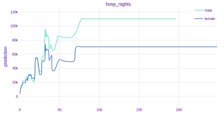
FIGURE 6.5: Partial Dependence Profiles for number of nights spent in the hospital broken down by gender

Among patients who spent a few nights in the hospital, gender is not important for the amount of prediction. This rule begins to change after exceeding 30 nights. The PD profile for men has significantly higher values compared to the women’s profile, despite the fact that variable age doesn’t show much influence on the model. After exceeding 70 nights in the hospital, this variable does not affect the result returned by the model on average.

6.5 Instance Level Explanations

6.5.1 Business approach

In this subsection we will try to show the application of explanatory methods in the business approach. Selected observations are:

1. the person with the best estimated cost among people with results greater than 3000,
2. the person for whom the model predicted the highest cost of all.

Finding the value of characteristics that increase or decrease the final result, diagnostics of the direction of changes or oscillations of the result in case of change of characteristics describing a person may be valuable information for insurance companies or other payers for medical services. Such conclusions may also be useful for the patients, who have decided to pay for medical care themselves. In further consideration, the selected observations will be called Patient 1 and Patient 2.

Values of explanatory variables for patients.

Variable	Patient 1	Patient 2
hospital_nights	0	52
phys_visits	4	6
home_days	0	0
feet_checked	-1-inapplicable	-1-inapplicable
non-phys_visits	1	0
disposition	household	household
outpatient_visits	0	1
age	58	59
race	1-white	1-white
sex	2-female	1-man
edu	other	bachelor’s degree
diab_disease	1-yes	0-no
art_disease	1-yes	1-yes
ast_disease	0-no	1-yes
press_disease	0-no	0-no
heart_disease	1-yes	1-yes
real expenses	3882$	143457$
prediction	3886.8$	147178.5$

6.5.1.1 XIA for the best prediction

• XIA for the best prediction using Break Down Plots

Break-down plots show how the contribution of individual variables change the average model prediction to the prediction for observation.

The patient has 58 age, which alone increase average total cost by 574.177$ and the gender is female which decreases average total cost by 140. 72$. Her total number of office-based visits is 4, which increase average total cost by 574.177$. She suffers from arthritis what increase average total cost by 677.868$ but she is not diagnose to diabets, astma or high blood preasure which decrease final result. Her status of education is unknown, what increase total cost. The fact that she didn’t spend any night in the hospital decrease average total cost by 1343.271$. And also, she didn’t benefit from home medical services decrease average total cost by 386.772$.

• XIA for the best prediction using Shapley Values

To remove the influence of the random ordering of the variables in brake down results we can compute an average value of the contributions.

The plot shows that the most important variables, from the point of view of selected observation is number of days in home protected by medical servises, asthma disease or arthesis disease.

For this observation number of days in home protected by medical servises equals 0 decreases average total cost by 158.37$. A similar effect is achieved by the fact of not using outpatient visits, what decreases final medical cost by 134.79$.This woman hasn’t spent any night in the hospital, which reduces average total cost prediction by 47.11$. Unfortunately, the patient suffers from arthesis disease which increases average medical costs by 80.9 $, but fact, that she has no disease like asthma, decreases average response by 137.77$.

As said before, analised patient is a woman, what decreases average response by 77.37$. Her age is 58 what has positive impact on prediction and increase average total cost by 53.54$.

• XIA for the best prediction using LIME

The key idea behind this method is to locally approximate a black-box Gradient-Boosting model by a K-lasso interpretable model.

According to the LIME method, the plot suggests that spending any night in hospital reduces the estimated cost by 725.64$. Much greater, also the negative impact has a variable which telling that that patient didn’t benefit from home medical services, which total cost by 14072.46$. Having no outpatient visits also reduces final result by 4342.74$. Patient analysed is not diagnose the diabetes disease,which decrease response by 1518.18$. Variables that increase the cost of medical services are the total number of office-based visits greater than 3 and the age of the analyzed person greater than 54.

The first explanation concerns the observation for which the expenditure was small and the model overestimated it. Brake Down plot and Shap Values plot returns results that are intuitive. Below is a diagnostic plot model. For large cost values the rest is positive and for small ones negative, which suggests that the model in general works well, but it pulls the predictions to average.

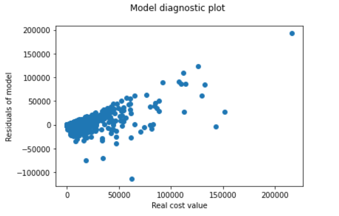
FIGURE 6.6: Model diagnostic plot

6.5.1.2 XIA for for the highest prediction

• XIA for the prediction with the largest cost using Break Down Plots

The patient spending 52 nights in hospital, which increase average total cost by 65749.48$. Having 59 age, increase average total cost by 16986$ and the fact that gender is male increase average total cost by 15105$. His status of education is bechelor degree, what increase total cost 1887$. Despite he is not diagnose to diabets and high blood preasure which decrease final result, he suffers from heart disease which also decrese avarage response.

• XIA for the prediction with the largest cost using Shapley Values

As we expected, for the observation that generated the highest predictions, most of the variables have an additive effect on the final result. The graph shows that the greatest influence on the final value of the average prediction is race, disposition and number of night in hospital.

For this patient, the fact that he’s a white man raises the average estimates by 21213.64$. Living in a household increases the average prediction by 17353.7$. Spending 52 nights in hospital increase average response by 16483.7$, likewise number of physical visits equals 6, raises average total prediction by 4518$.

• XIA for the prediction with the largest cost using LIME

The LIME method also returns a positive influence on the final prediction for most variables. The chart shows that spending 52 nights in hospital increases treatment costs by 38817 $. The total number of office-based visits greater than 3 also has a positive impact, increasing the prediction by 6866.85 $. The age of a patient over 54 also significantly increases medical costs. Among the variables reducing treatment costs ,was the total number of days in home health care equal to 0.

6.5.1.3 XIA for both predictions using Ceteris Paribus Profiles

In this chapter we will use Ceteris-paribus profiles for instance level explanations. Ceteris-paribus profiles show how the model response would change if a single variable is changed. So here we will be checking how would the model prediction change, if we change only one property of the patient and how it influences our model

In the plot below we have selected features that behave differently between those two patients. Those features are sex, age, hosp_nights, phys_visits, feet_checked and outpatient_visits.

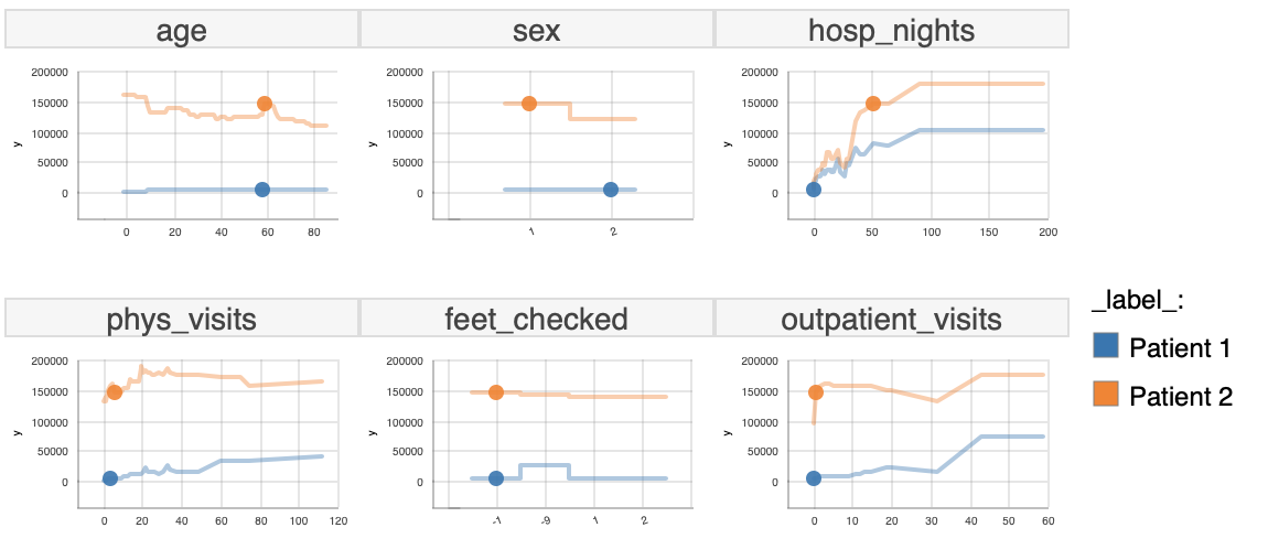
FIGURE 6.7: Ceters Paribus plot for selected 6 features

What can be observed is that the plots for Patient 2 are higher on the expenses axis, because of the fact that Patient 2 has higher costs, but the curvature of both curves is quite similar with some small differences like for the feet_checked variable.

In later subsections we will dive more into those differences.

• Comparing differences between patients based on sex

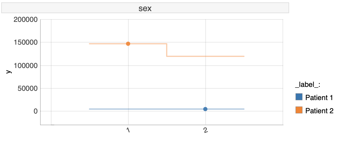
FIGURE 6.8: Ceters Paribus plot for SEX

As we can see, our explanation model tries to predict what would have happened if the patient would have a different sex. For patient 1 there would be no difference in the predicted value, but for patient 2 the change of sex implicates reduction or an increase in predicted costs. This means, that if there would exist a different patient with similar as patient 2 symptoms and attributes but with different sex, the predicted cost would be different.

• Comparing differences between patients based on age

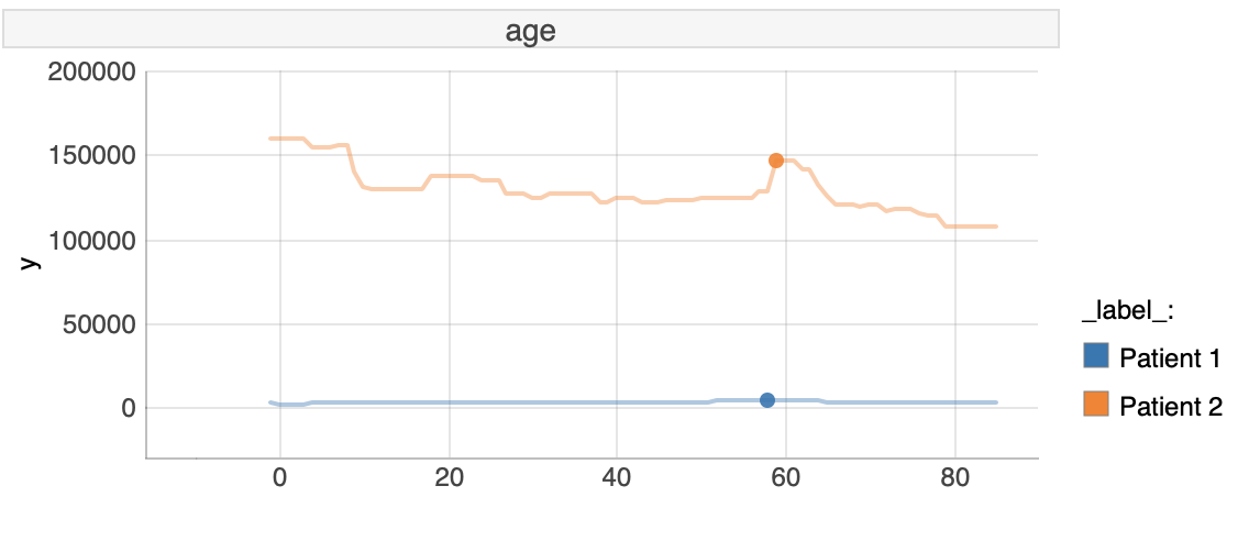
FIGURE 6.9: Ceters Paribus plot for AGE

In this section we will investigate age. Here both patients are almost the same age, 58 and 59 respectively for Patient 1 and Patient 2. For patient 1 there is no influence of age on the expenses, but for patient 2 there is an influence of this variable on predicted expenses. For patient 2 being around age of 60 and below age of 10 implicates a rise in predicted costs and for different possible ages it is almost constant. This means that for a patient with similar attributes as Patient 2, being around age 60 and below age of 10 implicates higher medical expenses, according to our model.

• Comparing differences between patients based on number of nights associated with hospital discharges

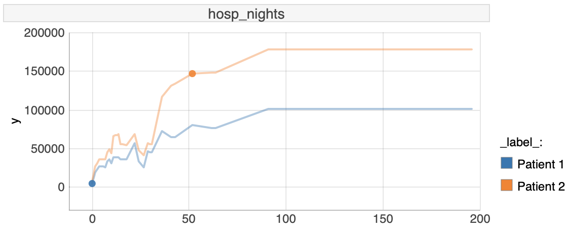
FIGURE 6.10: Ceters Paribus plot for hosp_nights

On the plot above for variable hosp_nights, both patients behave similarly, but with a different sensitivity. Patient 2, because of higher costs, is more sensitive in changes of the number of nights associated with hospital discharges. We can observe here, that hosp_nights equal to 0 implicates that the expenses are also equal to 0. With the increase of hosp_nights the expected expenses also rise until value of hosp_nights equal to 100, then expenses are constant. It is worth mentioning that not always hosp_nights equal to 0 means that there are no expenses.

6.5.2 Instance Level Explanations - instance specific approach

Here we will try to show the results of explanatory analysis methods for selected instances of data, that is for specifically selected different people with different backgrounds, races, age and sex. The main idea behind this is to see how the model responses are different for different gender, race and age and which variables influence the model for each patient.

A review of selected variables

Variable	Patient 1	Patient 2
hospital_nights	0	3
phys_visits	12	8
home_days	0	0
feet_checked	2-yes	-1-inapplicable
non-phys_visits	0	6
disposition	household	household
outpatient_visits	0	3
age	71	34
race	2-black	1-white
sex	1-man	2-female
edu	no degree	no degree
diab_disease	1-yes	0-no
art_disease	1-yes	0-no
ast_disease	0-no	0-no
press_disease	1-yes	0-no
heart_disease	1-yes	0-no
real expenses	2263$	16268$
prediction	8779$	24373$

So as in table above we will investigate 2 patients, where one is of age 71 and with several illnesses, where the second one is of age of 34, different sex and without illnesses.

6.5.2.1 XIA for Patient 1

For this patient our model had predicted expenses equal to 8779$, where the real expenses were 2263$. This means that for this observation our model overestimated the expenses by 6516$.

• XIA for Patient 1 using Break Down Plots

Here we will be showing explanations using Break-down plots and explain the contribution of individual variables on the prediction.

The first patient is of age 71. The age variable in comparison to previous explanations should have significant impact on the prediction but not in this case. For this case, patients age increased the predicted expenses only by 141$.

The biggest influence on the prediction has variable phys_visits, which is the number of office-based physician visits. It alone was responsible for 4300$ of expenses. Also diabetes and an feet_checked (indicator whether the respondent reported having his or her feet checked for sores or irritations) have positive influence on the predicted expenses. These two observations increased the predicted cost bo 6000$.

Variables hospital_nights, non-phys_visits and edu have most significantly negative influence on the prediction and lowered the predicted expenses by 2400$. The reason behind this, might be that our observation has 0 hospital_nights.

• XIA for Patient 1 using Shapley Values

We can run explanatory analysis using shapley values for those patients. For Patient 1, all observations apart from home_disease_days have positive influence on the predicted value.

Top three variables with the highest influence are diseases, and 3 after them are number of vists related variables. These top 3 diseases alone increased the predicted cost by 1800$. Next 3 variables which indicated the number of visits, increased the expected cost by 1100$. This is very interesting observation that is telling us, that diseases are the most important reasons why our medical expenses rise.

• XIA for Patient 1 using LIME

Here we are using the LIME method for the explanations by approximating a complex model by a simpler one, which is easier to interpret.

In the plot above, we can observe that for Patient 1, the prediction is heavily influenced by hosp_nights, which is the number of nights in a hospital. It influences negatively the prediction, thus lowering the expected costs. The same is for home_disease_days variable, which also negatively influenced the prediction. The reason behind such a result could be that our patient has 0 nights in a hospital and 0 home days. On the other hand, number of office-based physician visits has a positive impact on the models prediction, causing the expenses to be higher.

6.5.2.2 XIA for Patient 2

For this patient our model had predicted expenses equal to 24373$, where the real expenses were 16268$. This means that for this observation our model overestimated the expenses by 8105$.

• XIA for Patient 2 using Break Down Plots

Here we will be showing explanations using Break-down plots and explaining the contribution of individual variables on the prediction.

The second patient is of age 34. In this case the most significant influence on the prediciton have variables hospital_nights and outpatient_visits which are responsible for almost 17k of expenses. Other variables that also influence the prediction are phys_visits and non-phys_visits.

Other variables have very small or small but negative influence on the prediciton.

This is quite interesing, because the variables that are making the expenses to go higher are pure number of visits in hospital or by some medical employees.

Here in comparison with patient 1, hospital_nights variable has positive influence on predicted cost, where for patient 1 it was negative. This paient has hospital_nights greater then 0, which could be the reason behind such a change.

• XIA for Patient 2 using Shapley Values

We can run explanatory analysis using shapley values for those patients. For Patient 2, all observations have positive influence on the predicted value.

Here just as for the first patient, top two most important variables are diseases. There are also 2 other diseases with slightly smaller influence, but still a significant one. What is interesting here, diab_disease and art_disease being 0 influenced the result the most, where for patient 1 they were equal to 1 and were also in top influencial variables.

• XIA for Patient 2 using LIME

For Patient 2, the explanations received using LIME method show us, that number of nights in a hospital have the highest positive influence on the prediction. It means that number of nights in a hospital for this patient is making the medical expenses higher for him, while home_disease_days variable is making the expenses lower. Other variables like phys_visits, non-phys_visits and outpatient_visits influence the prediction making the expenses to rise.

Such results are very natural and are easy to understand by anyone investigating such a prediction. We can also see a difference in comparison to the first patient, where number of nights in a hospital were making the expenses lower, because he had 0 of them.

6.5.2.3 XIA for Patient 1 and Patient 2 using Ceteris Paribus Profiles

In this chapter we will use Ceteris-paribus profiles for instance level explanations and see how would the model prediction change, if we change only one property of the patient and how it influences our model. We will see if there are any clear differences between patients and how our model is treating each one of them.

• Comparing differences between model predictions for Patient 1 and 2 for diffenret properties

Here we present a plot, on which we list all variables that are interesting to investigate. We will try to investigate, how the model behavior changes for each patient, when their properties change. One thing to be aware of, both patients have different predicted expenses, so we will be mainly interested in the curvature of the plots.

FIGURE 6.11: Ceters Paribus plot for six variables

As shown on the plot above, each value of the patient property influences a bit differently the outcome of our model. Patient 2, who has higher expenses, has higher values on our plots, but the dynamics of those plots for both patients are very similar.

• Comparing differences between patients for number of nights associated with hospital discharges

Here we have chosen the variable that describes the number of nights the patient has spent in a hospital.

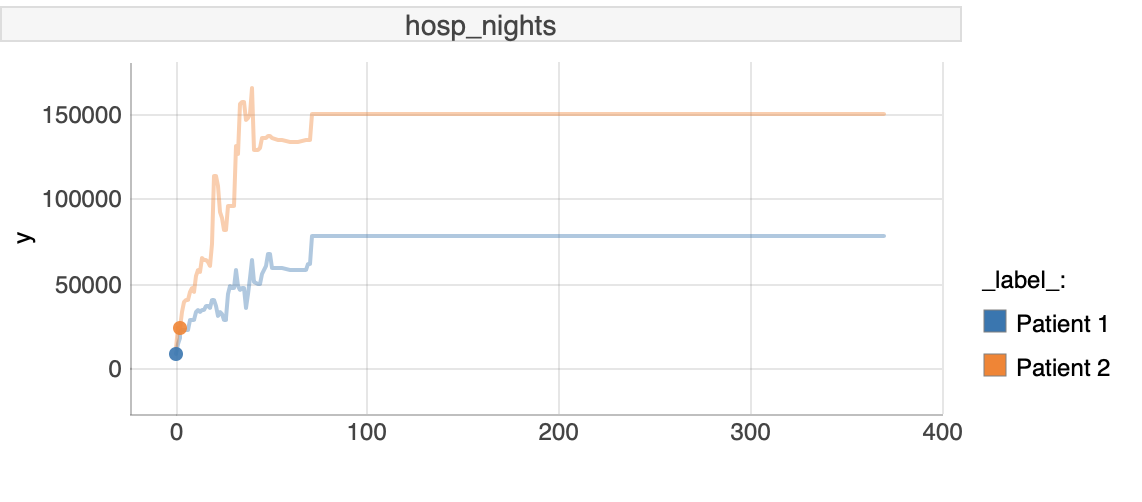
FIGURE 6.12: Ceters Paribus plot for hosp_nigths

For this property of our patients, we would like to show how the model responds, when values of the number of nights associated with hospital discharges influences the predicted costs.

The number of nights influences the expenses for patient 1 and 2 similarly, but with different power. Patient 2, due to having a higher prediction of expenses is being influenced more than patient 1, but with the same dynamic. This shows that our model treats both patients similarly.

• Comparing differences between patients for variable of number of office-based physician visits.

Here we have chosen the phys_visits variable which is the number of office-based physician visits.

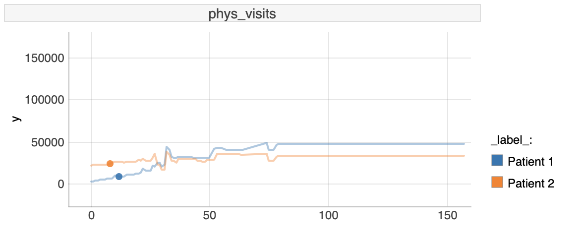
FIGURE 6.13: Ceters Paribus plot for phys_visits

In this case we can notice an interesting influence of the variable phys_visits. For patient 1, the higher the number of office-based physician visits, the higher would be the predicted outcome of our model.

This is different for patient 2, for whom the predicted value is not changing, sometimes it is even declining. This is very interesting, because it tells us, that Patient 2, which is younger is almost not influenced by the number of office-based physician visits, while the older patient 1 has higher expenses with higher number of those vists.

6.6 Summary and conclusions

Undoubtedly, explanatory methods open up new opportunities in the business sector as well as in the diagnostic model and exploration. The data on which the analysis has been carried out covers the entire population of the United States of America. Depending on age, education, gender, and many other agents, people take different approaches to looking after their health.

The analyses presented in the above chapter have provided conclusions that may be useful in various areas.

Model-level exploration showed that it is worthwhile to study the impact of variables on each other, as this may show more complex relationships. In our case, the SEX variable, which doesn’t show much impact affects the most important variable almost twice.

Explainability methods can certainly work in the business sector. Case analysis at the instance level allowed to compare the behavior of the model for people with different characteristics. An interesting observation is undoubtedly the fact, that the total medical cost was strongly influenced by a variable of the number of days in the hospital, rather than the patient’s demography or medical history itself. Perhaps, it would be worthwhile for financial institutions to make a two-stage analysis to estimate the final result. First is to estimate the number of days spent in hospital or at home with illness based on demographic factors and medical history. The second is, to use these results for further calculations. It could contribute to a more accurate assessment of the costs generated and be more beneficial for companies.

Explanation methods have helped to understand why the model often overestimates observations and to diagnose that the model pulls observations to average. This has facilitated further interpretation of the results.

We also paid attention to people who differ in their state of health and age. In this case too, the number of visits to the hospital turned out to affect the outcome. Nevertheless, for these observations, the health condition also had a strong impact, both for the young and the elderly. The explanatory methods at the instance level gave the picture that people care about their health differently.

6.7 References

Przemysław Biecek, Tomasz Burzykowski, Explanatory Model Analysis: Explore, Explain and Examine Predictive Models, https://pbiecek.github.io/ema/preface.html

\begin{document}

\begin{markdown}