Breaking Down of Model Predictions for lm models

Breaking Down of Model Predictions for lm models

# S3 method for lm
broken(model, new_observation, ..., baseline = 0,
  predict.function = stats::predict.lm)

Arguments

model	a lm model
new_observation	a new observation with columns that corresponds to variables used in the model
...	other parameters
baseline	the orgin/baseline for the breakDown plots, where the rectangles start. It may be a number or a character "Intercept". In the latter case the orgin will be set to model intercept.
predict.function	function that will calculate predictions out of model (typically predict or betas)

Value

an object of the broken class

Examples

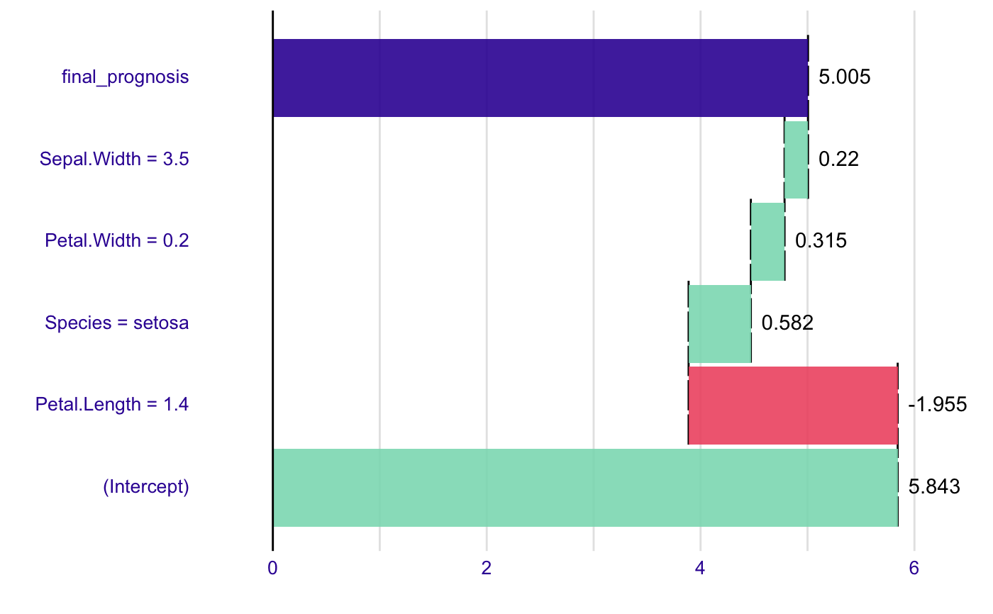
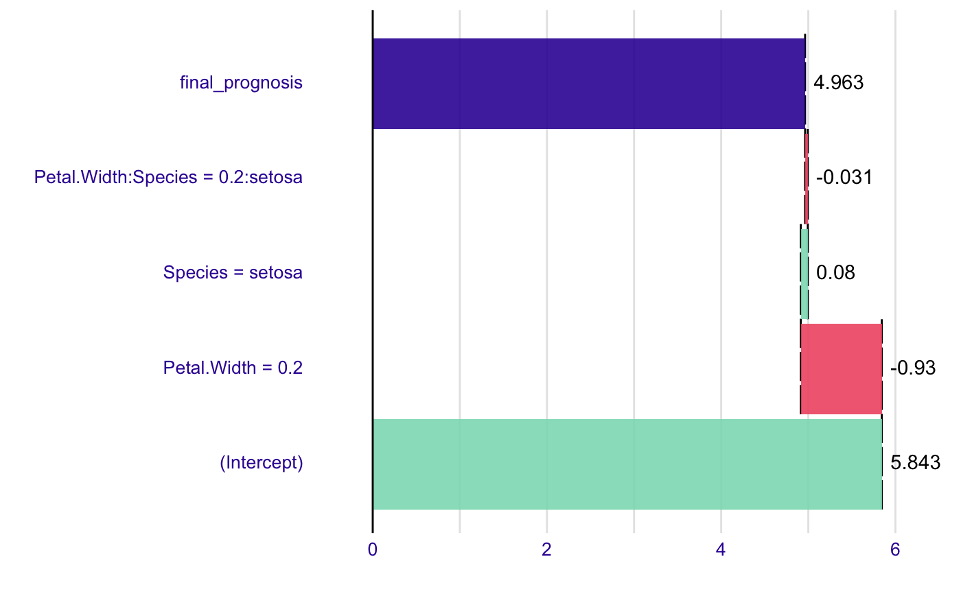
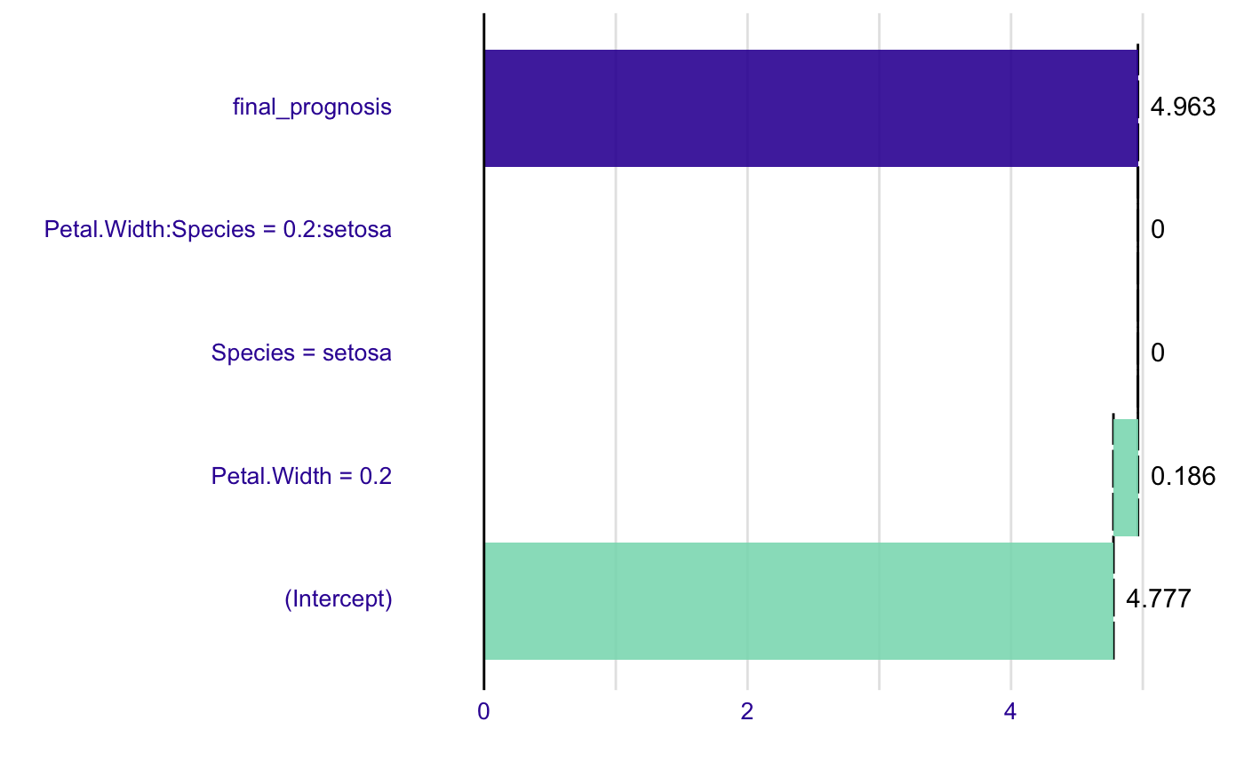
model <- lm(Sepal.Length~., data=iris)
new_observation <- iris[1,]
br <- broken(model, new_observation)
plot(br)

# works for interactions as well
model <- lm(Sepal.Length ~ Petal.Width*Species, data = iris)
summary(model)
#> 
#> Call:
#> lm(formula = Sepal.Length ~ Petal.Width * Species, data = iris)
#> 
#> Residuals:
#>      Min       1Q   Median       3Q      Max 
#> -1.47583 -0.29891 -0.04508  0.25075  1.32892 
#> 
#> Coefficients:
#>                               Estimate Std. Error t value Pr(>|t|)    
#> (Intercept)                     4.7772     0.1735  27.541   <2e-16 ***
#> Petal.Width                     0.9302     0.6491   1.433    0.154    
#> Speciesversicolor              -0.7325     0.4951  -1.480    0.141    
#> Speciesvirginica                0.4922     0.5379   0.915    0.362    
#> Petal.Width:Speciesversicolor   0.4962     0.7356   0.675    0.501    
#> Petal.Width:Speciesvirginica   -0.2793     0.6953  -0.402    0.688    
#> ---
#> Signif. codes:  0 ‘***’ 0.001 ‘**’ 0.01 ‘*’ 0.05 ‘.’ 0.1 ‘ ’ 1
#> 
#> Residual standard error: 0.4789 on 144 degrees of freedom
#> Multiple R-squared:  0.6768,	Adjusted R-squared:  0.6656 
#> F-statistic: 60.31 on 5 and 144 DF,  p-value: < 2.2e-16
#> 

new_observation <- iris[1,]
br <- broken(model, new_observation)
br
#>                                  contribution
#> (Intercept)                             5.843
#> Petal.Width = 0.2                      -0.930
#> Species = setosa                        0.080
#> Petal.Width:Species = 0.2:setosa       -0.031
#> final_prognosis                         4.963
#> baseline:  0 
plot(br)

br2 <- broken(model, new_observation, predict.function = betas)
br2
#>                                  contribution
#> (Intercept)                             4.777
#> Petal.Width = 0.2                       0.186
#> Species = setosa                        0.000
#> Petal.Width:Species = 0.2:setosa        0.000
#> final_prognosis                         4.963
#> baseline:  0 
plot(br2)