1.3 Setting up the environment

To enjoy a convenient R environment, we should follow the three steps below.

Install the basic R environment, which comprises an interpreter and a basic set of packages. This set alone offers enormous capabilities. It will be enough for most users to analyse data, draw plots and perform other typical tasks.
Install RStudio. It is a tool which facilitates working with the R software. It is not the only R editor out there, but seems to be the best solution. Similarly to R itself, the basic version of RStudio is free of charge.
Install additional packages with useful functions. There are over 7,000 packages available now! You do not have to install them all at once. You will sometimes need new functions from new packages as you work with R, and it is only then that you should install them.

Below, we present a short summary related to each installation stage.

1.3.1 Installing basic R environment

The source and binary R files are available for most operating systems, including all Linux and Unix distributions, Windows 95 or higher, and Mac OS.

At the time of this writing, the latest R version is 3.3.2. Each year in April, there is another major 3.x version appearing, which means that we will soon enjoy version 3.4.0. During the year, further subversions are released as need be. R is being developed quickly and we should update it at least once a year to get its latest version.

In order to install R, go to https://cran.r-project.org/, choose the operating system and download the binary file. The installation itself is as simple as clicking Next a few times. You can have a few versions of R installed at the same time. Keeping older versions of R may be useful when we want to reproduce the exactly same results in the future.

If you install R on a less typical platform, you can use the installation manual available at [49].

One useful feature of the R environment is that you can run it without installation. This means you can copy your R environment onto a CD, pendrive or external hard drive and run it on any other computer.

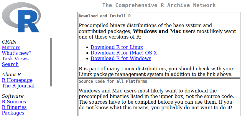
Figure 1.4: Website https://cran.r-project.org/. You can download the R program for the most popular operating systems.

It is hard to estimate the minimal system requirements for R. Its basic version runs without problems on older computers with 256 MB of RAM, Pentium processors and a few dozen MB of space on the hard drive. However, even though the basic version is “lightweight,” the installation of additional packages may require a few more GBs of RAM or hard drive space. Packages with big genomic data are particularly “heavy-weight.”

Those using R for compute-intensive analyses should rather use the R version for OS X, Linux or Unix. These systems manage memory more efficiently, which means that R works (slightly) faster. Unix-based systems also provide additional tools that allow multiple threads and other system mechanisms (such us fork()).

1.3.2 Installing RStudio

You can work with the basic R software alone, but working with an editor is much more convenient, especially when R is our main tool at work. Currently, the best editor available free of charge is RStudio – a tool developed by a company under the same name. This editor is available for Windows, Linux and OS X alike, supports many advanced packages and functions of R.

RStudio is a tool which makes working with R easier. It is an editor, version manager, and debugger that makes creating packages, applications or reports easier. You can live without it, but it certainly helps much. The latest version of RStudio Desktop can be found at https://www.rstudio.com/.

An example screenshot from the program is shown in Figure 1.5.

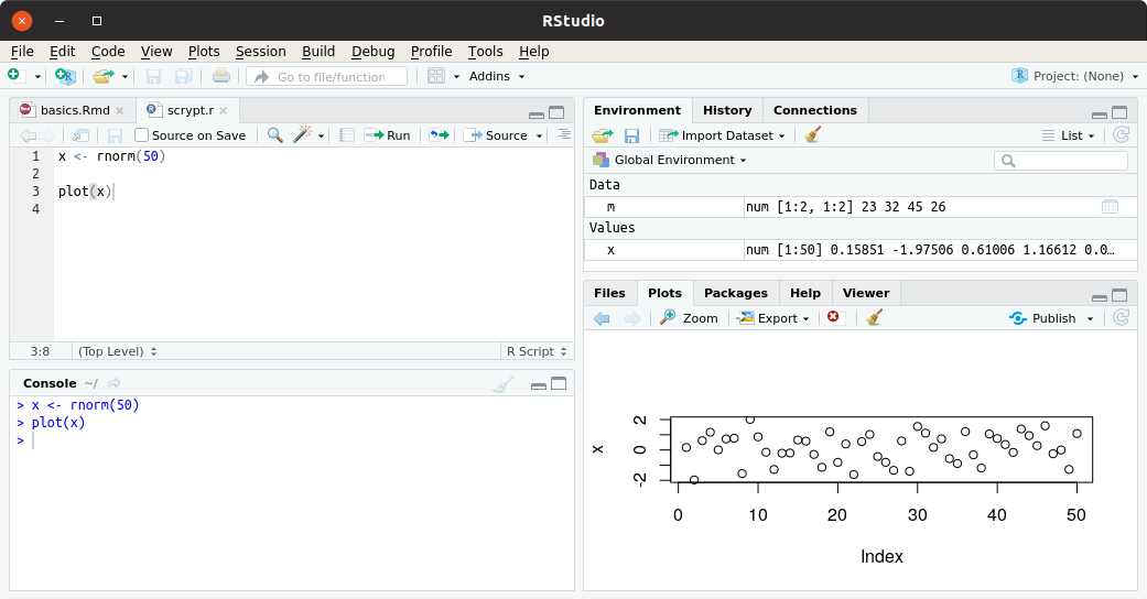
An example of the appearance of panels of the RStudio editor. The four panels show: window allowing to edit the code, window allowing to view variables loaded into the global R namespace, R program console, in which we can enter commands directly, and a window in which help files and charts are displayed by default.

Figure 1.5: An example of the appearance of panels of the RStudio editor. The four panels show: window allowing to edit the code, window allowing to view variables loaded into the global R namespace, R program console, in which we can enter commands directly, and a window in which help files and charts are displayed by default.

RStudio is very intuitive. Some of its interesting functions are:

Ability to automatically send the whole script or a piece of it to the R console. After selecting a given code snippet and pressing Ctrl-Enter, it will be executed in the R console.
Ability to manage multiple files and/or projects.
Support for knitr, Sweave and shiny packages, easy navigation among code fragments.
Support for R Notebooks, which allows interactive work with reports and running/updating code snippets.
Showing objects (names, classes, dimensions) available in the namespace.
Editor for data, functions and other R objects. When we click the name of a set present in the namespace, we can edit that object. It is often more convenient than using fix() or edit().
A simplified way to load data using a graphical interface.
Highlighting keywords and function names.
Contextual name auto-completion for functions, variables, properties, function arguments (when we start typing names, a list with matches appears).
Showing/hiding the code of functions or loops.
Support for creating and testing new packages.
Closing open brackets and quotes along with intelligent content highlighting.
Intelligent insertion of indentation combined with syntax recognition (i.e. indentation is added in loops, functions, etc.).
Interactive debugger.

RStudio Server is an interesting extension of RStudio Desktop. After installing it on a server, we can use R via our web browser. With the paid version, multiple users may open R at the same time.

Work in RStudio is much easier when you know some basic shortcuts. Below are those I personally find the most interesting. A very good description of RStudio alongside all keyboard shortcuts can be found at http://bit.ly/2d4B0Ix (so-called RStudio IDE cheatsheets). In the description below, Ctrl/Cmd means Ctrl for Windows/Linux and Cmd for OS X.

Ctrl/Cmd+Shift+C, comment a line or multiple lines.
Ctrl/Cmd+Enter, execute the highlighted code in the console.
Ctrl/Cmd+Up, show the history of commands.
Ctrl+L, clear the console.
Ctrl+1-9, switch between application windows.
Tab, autocomplete code – a very useful feature indeed.
Ctrl/Cmd+Shift+K, compile the current document.

1.3.3 Installing additional packages

Once we have the basic R environment in place, we already have access to various features. The real power, however, lies in the thousands of additional packages that contain further thousands of functions.

In order to use additional packages, we should follow these two steps:

Install a new package on the hard drive. You only need to do this once, the necessary files will be copied into the directory with packages. You can check the path to the directory with .libPaths().
Turn on the installed package in an active R session. This step must be performed every time we run the R environment. This will make the functions and datasets from the package available in the current session.

There are a few ways to install packages. We usually install them from the official CRAN repository (The Comprehensive R Archive Network). If the package we are interested in is available in CRAN, we can install it using install.packages().

For instance, the instruction below installs the Przewodnik package (Polish for Guide) directly from the CRAN repository alongside all the dependencies and datasets that we will use in this book. In order to install it, you only need to type the following code in the R console:

install.packages("Przewodnik")

Or choose Tools/Install packages... in RStudio.

Some packages are missing from the CRAN repository or are available in some older versions. For example, packages in CRAN are required to be 10 MB in size at most. Because of this limitation, greater packages must be stored elsewhere, typically in GitHub repositories. In order to install packages from GitHub, you can use the devtools:install_github() instruction.

For example, if you want to install the latest version of our Przewodnik package from the pbiecek Github repository, you can use:

devtools::install_github("pbiecek/PrzewodnikPakiet")

Apart from these two repositories, there are repositories for special purposes. For instance, many packages used in bioinformatical analyses can be found in the Bioconductor repository available at https://www.bioconductor.org/.

When we install a new package with data, functions and auxiliary files, they are stored on the hard drive of our computer. Before we can use them, however, we need to turn the package on. Each time we run the R platform, some basic packages such as base, graphics or stats are loaded. In order to use additional functions or datasets, we need to load (turn on) the package which contains them (assuming that the package is already installed). We use the library() instruction to turn packages on.

The instruction below turns on the devtools package. Once we execute this instruction, we can use the package without the need to add the devtools:: prefix.

library("devtools")

As we mentioned before, there are over 10,000 packages in the CRAN repository. It is difficult to find the feature we need in such a broad set. This is why we will use the following notation when using new functions: packageName::functionName(). ggplot2::qplot() means that the qplot() function can be found in the ggplot2 package. The index at the back of the book lists all functions both alphabetically and grouped by packages.

If we know the name of a function and want to find out the package that contains it, given that we do not have this book at hand, we can use the help.search() function. It will search through all installed packages and try to find the given name, or a function whose description contains the given search phrase. More information about this function and other means of searching information can be found in Section 1.4.

Once we have loaded the respective package, we can use its functions by providing their names. We can also explicitly name the package a function should come from. This might be useful when we have multiple functions with the same name in different packages. For example, both epitools and vcd packages contain an oddsratio() function, but each of them works in a different way. In order to specify the package, we can see the :: or ::: operators. The :: operator only allows referring to public functions of a package, whereas the ::: operator also accepts references to private functions. Both lines of code below use the seq() function from the base package. The second method is useful when there are conflicting names of functions coming from different packages.

seq(10)
base::seq(10)

If we do not use the :: operator while there are multiple functions with the same name in different packages, R will use the function from the package loaded most recently.