2.6 How to load and save data in various formats
In this subchapter, we will present how to load tabular data from various sources. We will discuss all kinds of formats, since we understand that people who use R have various needs. For typical cases, you will only need to read the first three sections that explain how to load data from packages, text files and Excel files.
Generally speaking, data sets can have various structures. They can be expressed as graphs, trees, they may describe photos or multimedia files. All of these structures can be loaded into R and analysed. Most of the time, however, the data sets that we work this have a tabular structure with columns and rows clearly marked. We will put focus on this sort of structure in the following subchapter.
2.6.1 Loading data from text files
Loading data from packages is the easiest case. You only need to turn the given package on using library(), and then use data() to load a given file. A single package can store multiple datasets, which is why packages are often used as storages of useful data.
One of such packages is the PogromcyDanych package (Polish for Data Busters). It contains various datasets which we use in the present book, such as cats_birds. Once we install the PogromcyDanych package, we only need two lines of code to use this dataset:
library("PogromcyDanych")
cats_birds <- read.csv("cats_birds.csv",sep=";",dec=",")
A new symbol for the dataset should appear in the Environment of RStudio. We can see the first few rows using the head() function.
head(cats_birds)## species weight length velocity habitat lifespan team
## 1 Tiger 300 2.5 60 Asia 25 Cat
## 2 Lion 200 2.0 80 Africa 29 Cat
## 3 Jaguar 100 1.7 90 America 15 Cat
## 4 Puma 80 1.7 70 America 13 Cat
## 5 Panthera 70 1.4 85 Asia 21 Cat
## 6 Cheetah 60 1.4 115 Africa 12 CatThe cats_birds dataset contains 7 columns that describe various parameters of sample animals.
To show the list of all datasets in a given package, we can also use the data() function:
data(package="PogromcyDanych")2.6.2 Loading data from text files
Text files are a very popular format to store data. Their contents can be displayed in any text file, or in RStudio. They usually have the .txt, .csv (comma separated values) or .tsv (tab separated values) extension. In such files, subsequent column values are separated with some sort of separators, such as tabs, commas, semicolons, or other characters.
We will now analyse an example data set available on-line at http://biecek.pl/R/dane/cats_birds.csv. The file contents is presented below:
species;weight;length;velocity;habitat;lifespan;team
Tiger;300;2,5;60;Asia;25;Cat
Lion;200;2,0;80;Africa;29;Cat
Jaguar;100;1,7;90;America;15;Cat
Puma;80;1,7;70;America;13;Cat
Panthera;70;1,4;85;Asia;21;Cat
Cheetah;60;1,4;115;Africa;12;Cat
Snow leopard;50;1,3;65;Asia;18;Cat
Swift;0,05;0,2;170;Eurasia;20;Bird
Ostrich;150;2,5;70;Africa;45;Bird
Golden eagle;5;0,9;160;North;20;Bird
Peregrine falcon;0,7;0,5;110;North;15;Bird
Gerfalcon;2;0,7;100;North;20;Bird
Albatross;4;0,8;120;South;50;Bird
We can see that the file contains a table of values separated with semicolons. The first row is the header with column (variable) names:
species;weight;length;velocity;habitat;lifespan;team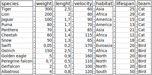
Figure 2.16: The logical structure of the cats-birds.csv file.
read.table() function. It has many parameters which are described in detail later. In the example below, the table of values that we loaded is assigned to the cats_birds symbol using the <- symbol.
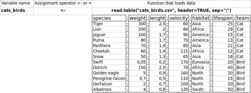
Figure 2.17: Logical structure of reading data from a file.
cats_birds <- read.table(file="http://biecek.pl/R/cats_birds.csv",
                         sep=";", dec=",", header=TRUE)
Data can be loaded from a file located on a hard drive, or downloaded directly from the Internet. In this case, we need to specify the following arguments:
file="http://biecek.pl/R/cats_birds.csv", i.e. text file path,sep=";", which defines the separator character,dec=",", which defines the decimal point; usually a dot, but can also be a comma, as shown in this file,header=TRUE, which informs that the first row contains headers and not values.
To find out whether data has been loaded correctly, we can again use the head() function. Alternatively, you can also use the Environment tab in RStudio, as shown in Figure 2.18.
head(cats_birds)## species weight length velocity habitat lifespan team
## 1 Tiger 300 2.5 60 Asia 25 Cat
## 2 Lion 200 2.0 80 Africa 29 Cat
## 3 Jaguar 100 1.7 90 America 15 Cat
## 4 Puma 80 1.7 70 America 13 Cat
## 5 Panthera 70 1.4 85 Asia 21 Cat
## 6 Cheetah 60 1.4 115 Africa 12 Cat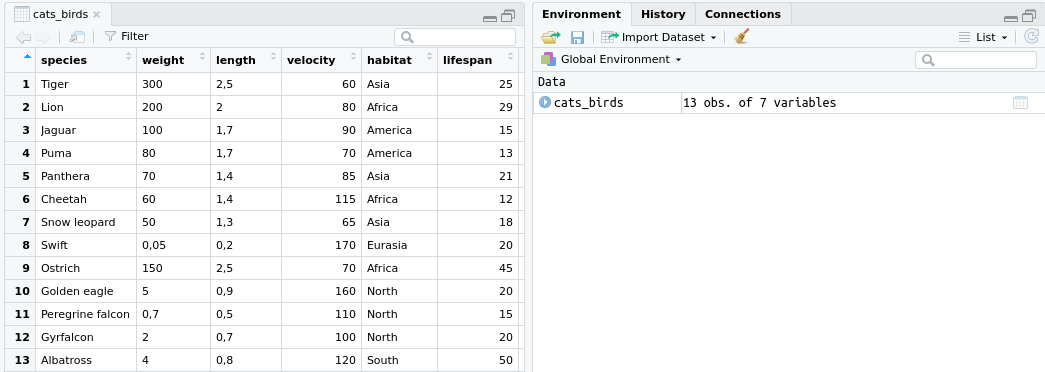
Figure 2.18: Table preview with data in RStudio.
Loading big files with
read.table()can take a lot of time. In such cases, you may consider using thedata.table::fread()function, which is much faster and has a similar number of parameters.
2.6.2.1 read.table() in detail
Unfortunately, there is no single universal format to store data in text files. Separators, decimal points, comment lines or strings can be defined with various characters.
The read.table() function is able to load data written in virtually any format. It is, however, only possible with a major number of additional options. The declaration of read.table() is as follows:
read.table(file, header=FALSE, sep="", quote="\"’", dec=".",
           row.names, col.names, as.is=!stringsAsFactors,
           na.strings="NA", colClasses=NA, nrows=-1, skip=0,
           check.names=T, fill=!blank.lines.skip, strip.white=F,
           blank.lines.skip=T, comment.char="#", allowEscapes=F,
           flush=FALSE, stringsAsFactors, encoding = "unknown")
In the utils package, there are four other functions that work in the same way, but have other default values.
read.csv(file, header=TRUE, sep=",", quote="\"", dec=".",
         fill=TRUE, comment.char="", ...)
read.csv2(file, header=TRUE, sep=";", quote="\"", dec=",",
          fill=TRUE, comment.char="", ...)
read.delim(file, header=TRUE, sep="\t", quote="\"", dec=".",
           fill=TRUE, comment.char="", ...)
read.delim2(file, header=TRUE, sep="\t", quote="\"", dec=",",
            fill=TRUE, comment.char="", ...)
If we saved the data in the CSV format using the Polish version of Excel, semicolons will be used as separators, and commas as decimal points. In such cases, the read.csv2() function is most suitable. If we use the English version of Excel, dots will be used as decimal points, and the read.csv() function will be a better solution.
Table 2.2 presents the descriptions of read.table() arguments. The English version of these descriptions can be found in the help file: ?read.table. As can be seen, there are many arguments, and we suggest you read about each of them at least once.
| Function | Description |
|---|---|
| \(\texttt{file}\) | String value. It is the only obligatory argument which must be explicitly provided. Its value is the file path where the data is stored. We can provide a local file, or a file from the Internet by providing the URL that specifies the server and directory of the file. This field can also specify a connection or a socket. If we provide “clipboard” instead of a file name, data will be read from the system clipboard, which is a convenient way of loading data from various MS Office programs. |
| \(\texttt{header}\) | Logical value. If it is \(\texttt{TRUE}\), the first argument will be treated as a list of columns. If this argument is not provided, and the first line contains one field less than other lines, R will automatically treat this line as the header. |
| \(\texttt{sep}\) | String value. The given string will be treated as the field separator. The default "" value treats each whitespace (single space, multiple spaces, tabulator, new line) as a separator. |
| \(\texttt{quote}\) | String value. It defines the character that represents the decimal point. If data is saved according to Polish standards, the comma sign “,” is the decimal point. |
| \(\texttt{row.names}\) | A vector of strings or a single number. If a vector of strings is provided, it will be treated as the names of subsequent rows. If this argument is a number, it will be treated as the ordinal number of the column in the loaded file that contains row names. If the data contains a header (i.e. \(\texttt{header=TRUE}\)) and the first line has one field less than other lines, then the first line is automatically treated as a vector with row names. |
| \(\texttt{col.names}\) | Vector of strings. Column names can be specified with this argument. If it is not provided, and the file does not contain a header, then subsequent column names start with the letter “V,” followed by increasing integer numbers. |
| \(\texttt{nrows}\) | Numerical field. Specifies the maximal number of rows to be read. |
| \(\texttt{skip}\) | Numerical value. Specifies the number of initial lines that should be ignored when reading the file. |
| \(\texttt{check.names}\) | Logical value. Specifies whether column names should be checked for correctness (i.e. without illegal characters or repetitions). |
| \(\texttt{as.is}\) | Vector of logical or numerical variables. By default, each field which is not converted into a real number or logical value is converted into a \(\texttt{factor}\) type variable. If the \(\texttt{as.is}\) parameter is a vector of logical values, then it indicates which columns can be converted into the \(\texttt{factor}\) type, and which cannot. A vector of numbers, instead, is treated as indexes of columns which should not be converted. |
| \(\texttt{na.strings}\) | Vector of strings. Indicates which values should be treated as \(\texttt{NA}\), i.e. which values are used for missing observations. Additionally, empty fields in columns with numerical or logical values are marked as missing observations. |
| \(\texttt{colClasses}\) | Vector of characters. Each character specifies the type of a single variable (column). Possible values are: (1) \(\texttt{NA}\) - default value, signifies automatic conversion, (2) \(\texttt{NULL}\) - a column will be skipped, (3) one of atomic classes (logical, integer, numeric, complex, character, raw, factor, Date or POSIXct). |
| \(\texttt{fill}\) | Logical value. If subsequent lines have different numbers of values, and \(\texttt{fill=FALSE}\) (default value), then \(\texttt{read.table()}\) will throw an error. If \(\texttt{fill=TRUE}\), shorter lines will be complemented with \(\texttt{NA}\) values to get the same line length. |
| \(\texttt{blank.lines.s}\) | Logical value. When \(\texttt{TRUE}\), empty lines will be skipped while reading the file. |
| \(\texttt{comment.char}\) | Character value. This character is treated as a comment character. All remaining characters in a given line after this character will be ignored. |
| \(\texttt{allowEscapes}\) | Logical value. When \(\texttt{TRUE}\), special escape characters are recognised. For instance, or are changed into tabulators or new line characters, respectively. \(\texttt{FALSE}\) (default value) means the text will be read literally, without any escape characters. |
| \(\texttt{stringsAsFactors}\) | Logical value. If \(\texttt{TRUE}\), strings will be converted into \(\texttt{factor}\) types. If \(\texttt{FALSE}\), they will be represented as strings. The default value is \(\texttt{TRUE}\). |
2.6.3 Saving data into text files
2.6.3.1 write.table() function
The write.table() function saves the values of a variable (atomic variable, vector, matrix or data frame) into a text file with a given formatting style. Below, we present the full declaration of this function:
write.table(x, file="", append=FALSE, quote=TRUE, sep=" ",
            eol="\n", na="NA", dec=".", row.names=TRUE,
            col.names=TRUE, qmethod=c("escape","double"))
Similarly to read.table(), the utils package features two functions that work in the same way as write.table(), but use other parameterisation of default arguments. Both functions are used to save data in the csv format.
write.csv(x, file = "", sep = ",", dec=".", ...)
write.csv2(x, file = "", sep = ";", dec=",", ...)
Table 2.3 describes all parameters of write.table() based on the help file: ?write.table.
| Function | Description |
|---|---|
| \(\texttt{x}\) | Object to save. Obligatory field. This object is usually a matrix or a data frame. |
| \(\texttt{file}\) | String value. Represents the path to the file in which the data should be written. This field can also represent a connection or a socket, just like \(\texttt{read.table()}\). Similarly, if we provide \(\texttt{"clipboard"}\) instead, the data will be saved into the clipboard. The " " value will print the object to the console. |
| \(\texttt{qmethod}\) | String value. Indicates how special characters should be marked. \(\texttt{"escape"}\) value is a C-style marking (with a backslash sign), while \(\texttt{"double"}\) value means a double backslash should be used instead. |
| \(\texttt{sep}\) | String value. This string will be treated as the separator of subsequent fields (the separator does not need to be a single character). |
| \(\texttt{eol}\) | String value. This string will be used as a line ending string. In Windows, the default value is \(\texttt{eol=" "}\). |
| \(\texttt{quote}\) | Logical value. \(\texttt{TRUE}\) means that \(\texttt{factor}\) types and strings will be surrounded with quotes \(\texttt{`"'}\). |
| \(\texttt{dec}\) | String value. This field defines the decimal point. By default, it is a “.” (dot). If the data is written in accordance with Polish standards, then the decimal point should be a “,” (comma). |
| \(\texttt{row.names}\) | Vector of strings or logical value. If a vector of strings is provided, it will be used to name subsequent rows. If a logical value is provided, it will specify whether row names should be written or not. |
| \(\texttt{col.names}\) | Vector of strings or logical value. If a vector of strings is provided, it will be used to name subsequent columns. If a logical value is provided, it will specify whether column names should be written or not. |
Below, we show a few examples of how to save a vector, number or a data frame into a file.
This instruction prints a vector of numbers onto the screen instead of saving it into a file:
write.table(runif(100),"")This instruction will write a vector into the clipboard:
write.table(1:100,"clipboard",col.names=FALSE, row.names=FALSE)This instruction will write a string into a text file:
write.table("Monday","c:/worstWeekday.txt")This instruction will save data in the CSV format into a file:
write.csv2(iris, file="forExcel.csv")Writing big objects of data.frame type into text files may be time-consuming. This happens due to the fact that formatting is switched between various columns that can present data of various types. R checks the type of each column and row, and formats the values based on their types. To speed up the process, it is sometimes better to convert the data into a matrix using as.matrix().
2.6.4 Loading and saving JSON data
Previously, we mainly discussed tabular data, but not all data can be saved as tables.
A universal and very flexible format used to transport various data sets is JSON (JavaScript Object Notation). It is frequently found in solutions that use Internet communication, such as REST services.
JSON is a text format (which means it is human-readable), describes data with a hierarchical structure (which is a very flexible solution), and is lightweight (does not take much space).
Below, we present a sample JSON file. It describes a two-element list whose first value is a string, and the second value is a table.
{ "source": "Przewodnik",
  "indicators": [
    {"year": "2010", "value": 15.5},
    {"year": "2011", "value": 10.1},
    {"year": "2012", "value": 12.2}
] }
In R, there are a few packages to read or write JSON files. The three most popular ones are RJSONIO, rjson and jsonlite. Each of them contains a toJSON() function which converts data into JSON, and a fromJSON() function which loads data from JSON.
The most stable option is the jsonlite package. Below, we only present some examples for this package.
From JSON to R: The data we load is initially a list. The structure is simplified into a data frame or a vector, where possible.
library("jsonlite")
fromJSON('{"source": "Przewodnik","indicators": [{"year": "2010", "value": 15.5},
         {"year": "2011", "value": 10.1},{"year": "2012", "value": 12.2}]}')
## $source
## [1] "Przewodnik"
##
## $indicators
## year value
## 1 2010 15.5
## 2 2011 10.1
## 3 2012 12.2From R to JSON: The example below shows how to convert the first two rows of the cats_birds data frame:
toJSON(cats_birds[1:2,])## [{"species":"Tiger","weight":300,"length":2.5,"velocity":60,"habitat":"Asia","lifespan":25,"team":"Cat"},{"species":"Lion","weight":200,"length":2,"velocity":80,"habitat":"Africa","lifespan":29,"team":"Cat"}]