Chapter 3 In search of factors influencing loan pay off
Authors: Weronika Skibicka, Martyna Poziomska (University of Warsaw), Adam Janowski, Maciej Bujalski (University of Łódź)
Mentors: Renata Grala, Bartosz Kozbial, Dawid Radwan (McKinsey & Company)
3.1 Introduction
Machine learning is playing an increasingly important role in the business world. Many large corporations are using machine learning algorithms as an aid in making various important business decisions. Most young people today decide to take out a loan, but not everyone pays it back. Banks in order to protect themselves against the situation that a client will not be able to repay entrusted to him credit uses machine learning algorithms, but as the data suggests we are not always able to predict whether the customer will pay it back.
3.2 Problem
The target of our project was to find out why some customers did not pay back the loan entrusted to them by the bank even though the algorithm algorithm claimed that they were able to repay it.
3.3 Data analysis
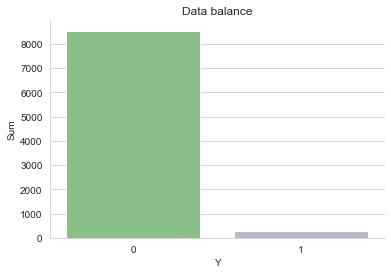
Given data included 294 variables with no missing values. There were 8830 records. However, our dataset was very unbalanced with only 3.32% of the people failing to pay off the loan.
All variables can be divided into 42 categories: Categories related to expenses: Alimony_Expenses, Pharmacy, ATM, Spending, Charity, Household, Decor, Delicatessen, Discounters, Child_Related, Electronics, Fast_Food, Hypermarket, Hobbies, Cafes, Cinema, Communication, Electricity, Fuel, Real_Estate, Renovation, Restaurant, Spa, Borrowing, School, Kindergarten, Theater, Telephone_and_TV_subscription, Flight_tickets, Train_tickets, Bus_tickets, OC/AC_insurance, Clothes, Medical_Services, Cleaning_services, Culture_Expenses Categories related to incomes: 500 plus, Alimony_Income, Retirement, Rent, Scholarship, Receipts, Salary
All the single category consists of 7 types of variables: The total amount related to category type customer expense/income in the last full month. The total amount related to category type customer expense/income in the last 3 months. The total amount related to category type customer expense/income in the last 6 months. The average amount related to category type customer expense/income in the last 3 months. The total number of related to category type customer expense/income in the last full month. The total number of related to category type customer expense/income in the last 3 months. The total number of related to category type customer expense/income in the last 6 months.
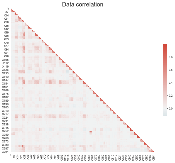
Variables were correlated only with those from the same category. No significant inter-category correlation has been spotted. Using the point-binary correlation coefficient, only 26 variables were correlated with the dependent variable Y.
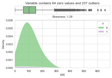
Looking at the distribution of an exemplary variable (all variables have a very similar distribution, showing the same tendencies and peculiarities), strong positive skewness and a very large number of outliers were visible.
3.4 Data engineering
To reduce the degree of freedom in the data, we decided to apply data engineering methods. The first step was to create new features by grouping and summing up the amounts or numbers of transactions in each group:
- Kids
- Health
- ATM
- home
- Food
- Transport
- Insurance
- Earnings
- Allowance
- Other
- Proportions receipts / expenses
with the time course: one month, three months, six months. Since there were a lot of accounts with zero values for expenses, we have exchanged all zero expenses value to 0.00(9), which is the highest unattainable expense value. Next, the following methods were used to extract information from the time course of the new features:
- Subtraction (first month - third month, third month - sixth month)
- Division (first month / third month, third / sixth month)
- Linear approximation (fitting a linear function to those three values)
- Normalized subtraction (first month - (third month / 3), (third month / 3) - (sixth month / 6))
It might seem that subtraction itself is not a very sensible solution, and that normalized subtraction should be more intuitive, but the results for the models with normal subtraction were much better than those with the normalized, which learned nothing and were random. Ultimately, therefore, standardized subtraction was not taken into account in explaining the model decisions.
The last method was to use only the 6-month values as this trait was expected to contain the most information and still third the degree of freedom in the data.
3.5 Pipeline
The pipeline consisted of three steps:
- Data Engineering
- Resampling
- Model
In the first step, Data Engineering, all of the techniques described in the previous subchapter were tested. Next step, resampling included oversampling the target group with ROS and SMOTE and undersampling the non-target group with RUS. All of those were tested alone, as well as in combinations: ROS+RUS and SMOTE+RUS. Three model types were tested: Logistic Regression, Random Forrest and Gradient Boosting, all implemented in the SciKitLearn package.
Initially, the resampling ratio was fixed at 30%. With that, 75 combinations of the pipeline were tested. From those, consistantly best performing were combinations with Random Forest as model and SMOTE as a stand-alone resampling technique. Those models underwent testing with different resampling ratios and data engineering techniques, with resampling ratio varying between 10% and 50%. From those test, the models further described in the next subchapter were selected. Two best performing models utilized Subtraction and Six-months-only approach to data engineering, achievieng the F1-score of 27%.
3.6 Explanations
3.6.1 Permutation Feature Importance
Most of the created models were unstable in performance, i.e. very slight changes in parameters, such as changing oversampling ratio about 0.1%, resulted with massive performance variance. In such case, a single best-performing model, is created more by luck than the factual dependencies in the data, most likely making it not robust. Thus, the approach to create multiple models to discover important data features was selected. 26 models, with performance, measured by F1 scored, above 18% were created and analyzed through permutation feature importance to extract features that are repeatably most important, in order to further reduce the noise in the data. The models were created using several data-engineering techniques and oversampling ratio. All of the models, however, were Random Forrest Classifiers and used only SMOTE as an oversampling technique, since those proved to be most effective.| Subtraction | Division | Six Months | ||
|---|---|---|---|---|
| Both | 3 | 2 | 5 | 10 |
| Money | 4 | 2 | 5 | 11 |
| Number | 3 | 0 | 2 | 5 |
| 10 | 4 | 12 | 26 |
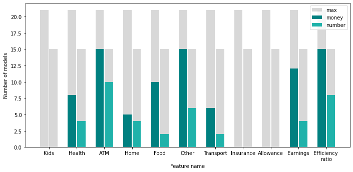
Out of 11 initial features, 5 were selected. A new model was trained using those five features, providing both: money and number information. While there was no significant improvement in the F1-score, there was also no significant drop. The input data was halved and the model retained the F1-score around 25% for the best hyperparameter selection.
3.6.2 SHAP
The standard method based on Shapley’s values was used to explain the predictions of individual bank customers. As none of the models differed significantly, the model that best suited the test dataset was selected for explanations. It is a Random Forest model which as an input receives the difference of amounts between individual months, and a feature representing the difference in the ratio of sums of payments to withdrawals between individual months.
Global SHAP explanations are shown in Figure 3.
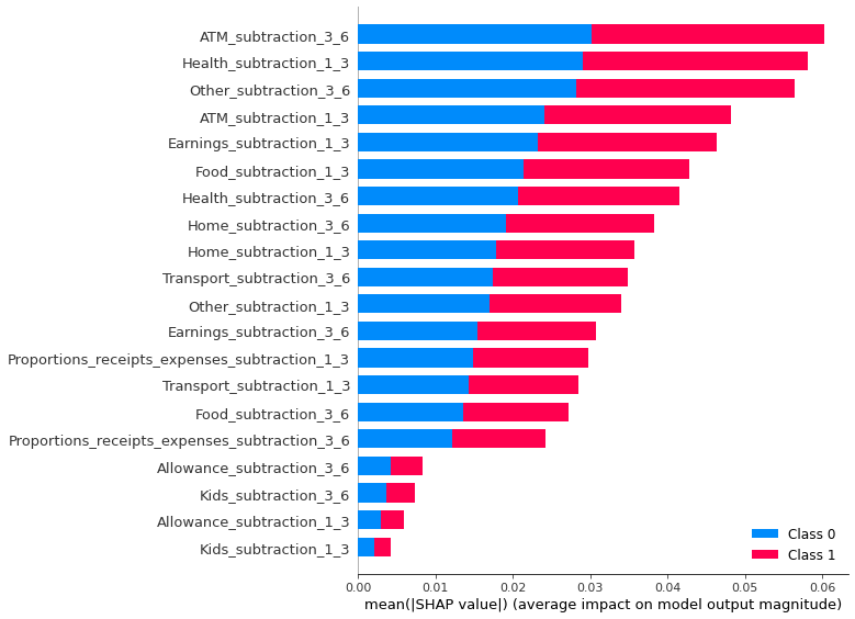
It is clear from global explanations that the three most important factors are ATM transactions, spending on health, and spending on other unnecessary things.
3.6.2.1 First case - model correctly predicted the lack of loan repayment.
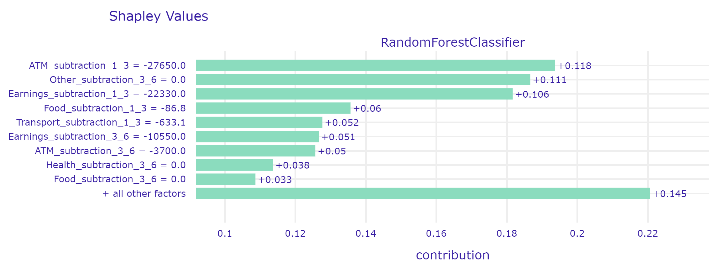
In this case, the model correctly predicted the default on the loan. He made his decision mainly based on ATM transactions, expenses for other unnecessary things, and the customer’s earnings.
3.6.2.2 Second case - model correctly predicted the lack of loan repayment.
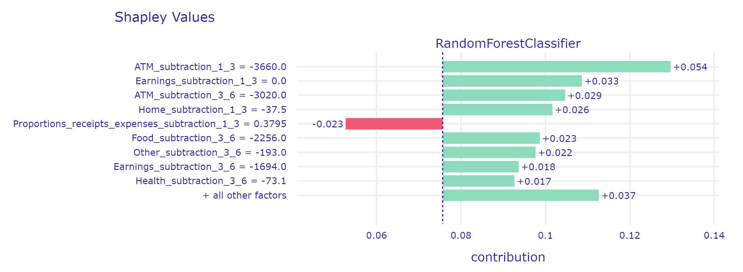
In this case, the model noticed that the client had attempted to stabilize his finances in the last three months (Proportions_receipts_expenses), which reduced his likelihood of defaulting on the loan.
3.6.2.3 Third case - the model incorrectly predicted the default of the loan.
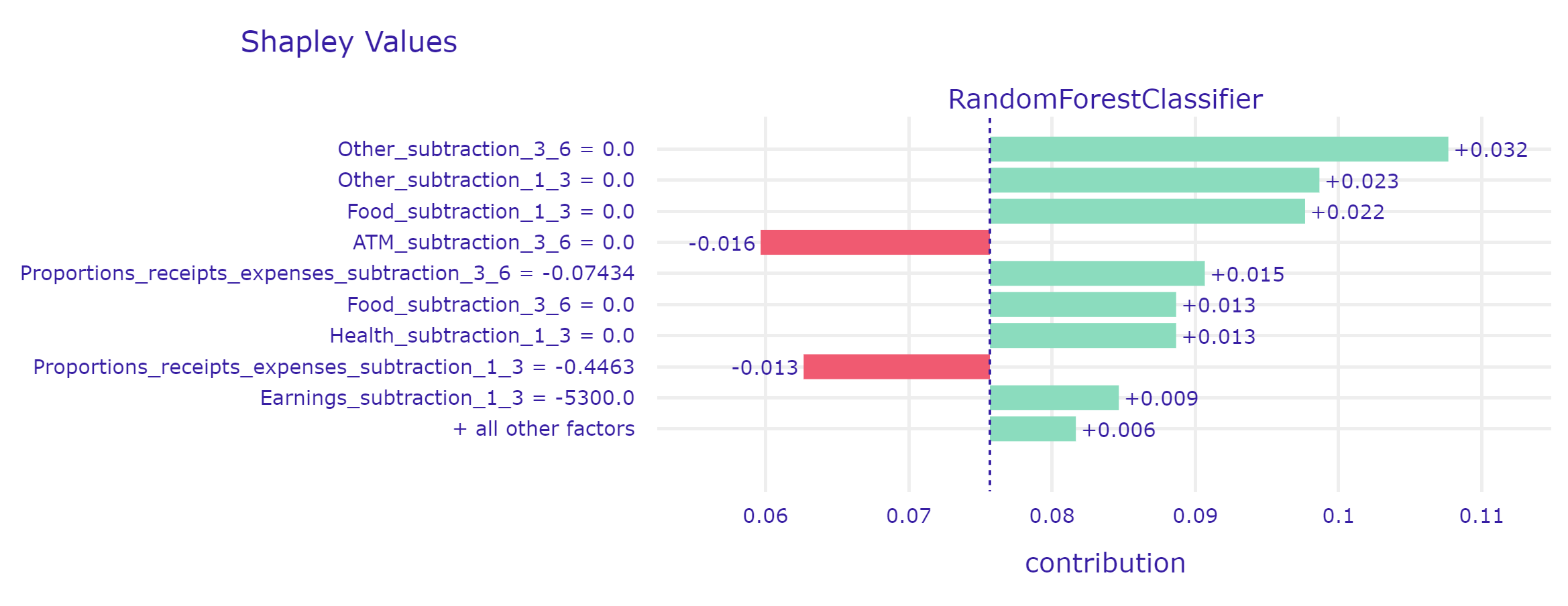
The big problem for the model are customers about whom there is virtually no information. Most likely, they set up an account with this bank just to take out a loan. In this case, using such a model does not seem to make sense, because the model does not have enough information to make a decision that will not be random.
3.7 Verification of explanations
It was decided to measure the correlation between the most important features across the models and expected behaviour as stated by the focus group. 30 individuals between 18-30 years old were asked to rank ten features in order from the most to least influential for a bank to grant someone a loan. Five of those features were the higher scoring features for models, as acquired in 5.2, with the exception of “Other”, which would recquire an explanation far exceeding the quick form of the questionare. Thus, the five features were: health expenses, food expenses, earnings, ATM transactions and efficency ratio. The other five, were made up, in order to noise up the questionare and protect the interests of Data Provider. They included: BLIK payments, subscription services expenses, physical activity expenses, entertainment expenses and non-fixed income. 6 of the responses were qualified as invalid, leaving 24 responses for analysis. All of the made up features had an average score below all of the original features, thus were disregarded in further proceedings. While ATM transactions have been constantly one of the most important features for the models, the focus group scored it as the least important from all of the original features. This might however be a problem with formulation of the question. The data, the models has been trained on was pre-selected, i.e. the model recieves information about the clients that have been granted a loan, and whether they paid them off. The contact point however is not a moment, when the client stops paying, but the moment they are granted a loan. Thus, the ultimate purpose of the task was not to grant them the loan. Such stated task however could lead to the the pre-selection model instead of the model at hand.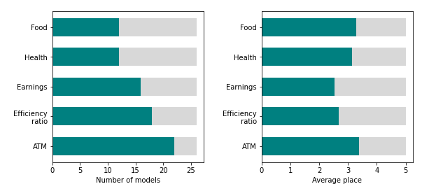
Features commonly associated with likelihood of getting granted a loan, like efficency ratio and earnings, would naturally be dilluded in this task. The model however seem to detect dependencies in those features, that passed through preselection.
## Summary