Chapter 2 Mincer earnings equation estimation
Authors: Michał Maciejewski (University of Łódź), Krzysztof Paprocki (University of Łódź), Piotr Żuber (University of Warsaw), Kamil Ruta (University of Warsaw)
Mentors: Michał Miktus (McKinsey), Justyna Pusiarska (McKinsey)
2.1 Introduction
The following chapter focuses on predicting current income of the client based on his features from the period of up to last six months. It will also be checked whether the experience (internship) measured by the client’s age has a significant positive impact on income. This is a reference to the Mincer equation: \(\log (Income) = \alpha_0 + \alpha_1 * Education + \alpha_2 * Internship + \alpha_3 * Internship ^ 2.\) Measurement of the client’s current income may be useful for the selection of personalized loan offers, offering types of bank accounts selected specifically for the client, deposits or a proposal to set up a specific investment portfolio. This chapter will try to explain what factors affect the customer’s income and how they affect it.
2.2 Data
The data contains 386 explanatory variables and 19 999 observations. The reference period for explanatory variables is up to six months before the estimation of current income. There are various explanatory variables for the same explanatory instance such as different time periods (one month, three months, six months) or various formats (nominal, share of expenditure, counts of activity).
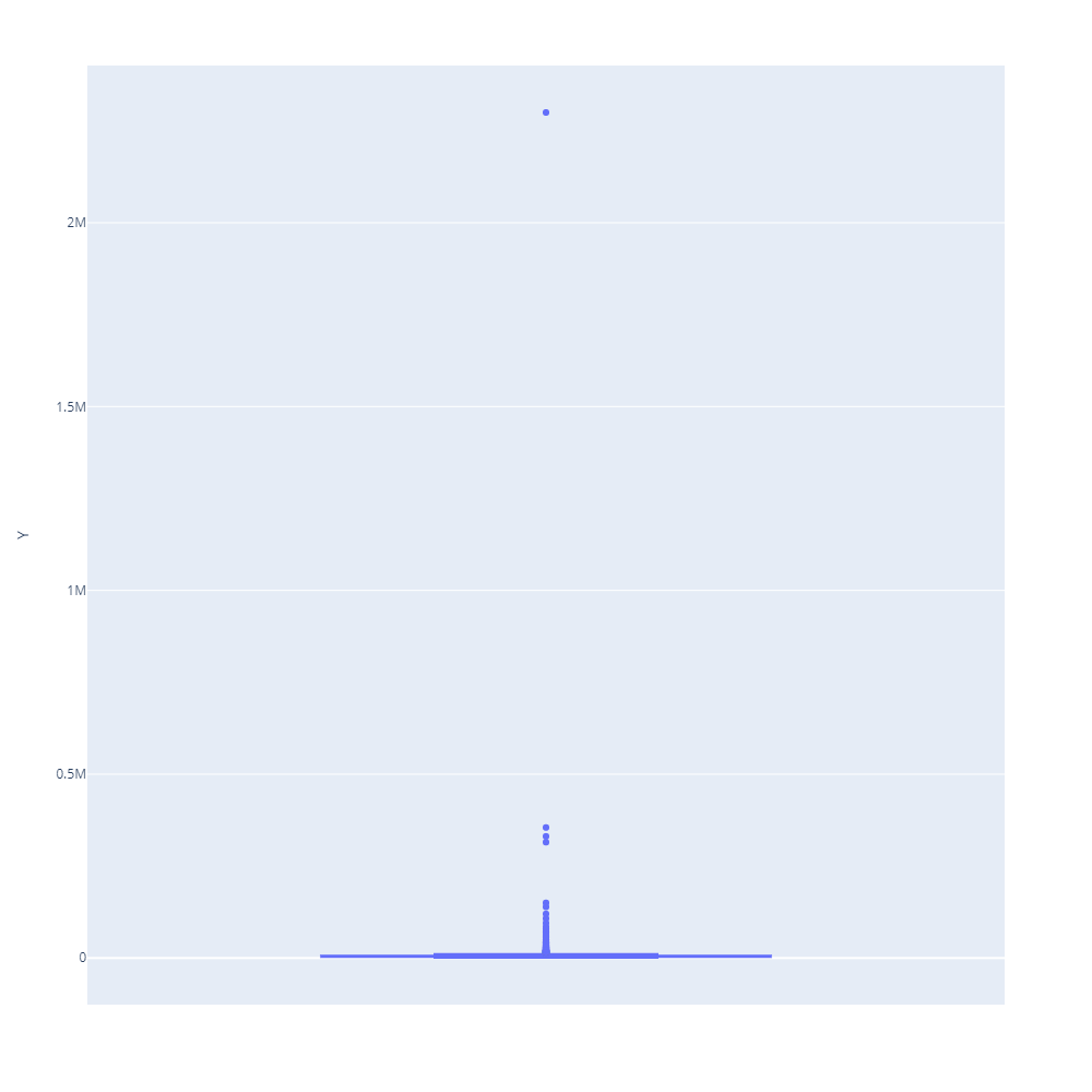
Plot 1. Box-plot of Y (current earnings)
Plot 2. Distribution of Log(Y)
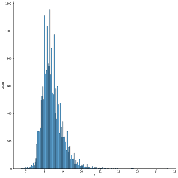
The box-plot points out multiple outliers across observations. Although the distribution plot of income might at first resemble a normal distribution, there is also visible skewness equal to 1.191, which alongside the outliers indicates that the distribution of income is clearly right-sided. The machine-learnig models might help to differ the outstanding observations from the others if their share common unique set of similar explanatory variables.
2.3 Models
The problem of predict income will be splited into two:
- Regression
- Classification
In regression the decimal log of income will be predicted and for the classification, the belonging to a certain income group. These groups represent belonging to a specific income group (1-lowest income, 5-highest income), created by breaking down observations into five quantiles. In this chapter, the focus will be on machine learning types of model, however at certain occasions those models and their explanations will be compared with linear model or Logistic Regression.
2.3.1 Basic Models Comprehension
In this section, the classification and regression models without optimized parameters will be compared with each other. It will also be tested whether the use of various scales are affecting the strength of prediction for the models. The blue metrics are marked as best among the models. Different types of machine-learning and more simplified models will be taken into consideration as follows:
For the Regression:
- Linear regression
- Random Forest Regressor
- XGBRegressor
- Lasso
- Ridge
For the classification:
- Logistic Regression
- Random Forest Classifier
- XGBClassifier
2.3.1.1 Regression
Tab.1 First Regression Models
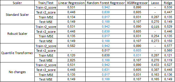
As for the regression, the results clearly indicate that Random Forest Regressor has the best scores across all different models except the situation where explanatory variables are adjusted using Quantile Transformer, however the linear models are less overfitted. Although XGBRegressor has worse scores than Random Forest Regressor it has slightly smaller problems with being overfitted and if optimized the results might be better than Random Forest Regression.
2.3.1.2 Classification
Tab.2 First Classification Models

The results of classification clearly show that although on the train sample Random Forest Classifier has better metrics, the XGBClassifier shows better results on the test sample. As expected, the Logistic Regression has worse scores regardless of the form of explanatory variables, but it much less overfitted than unoptimized machine-learning models.
The overall results of the metrics scores show that the simpler type of models have worse results on both train and test sample, however in general they are less overfitted than unoptimized machine-learning models. As shown, the results of both regression and classification problems indicate that although Random Forest type of machine-learning models can be better if not optimized, XGB type might be better as the parameters are optimized to reduce the problem of overfitting. The scale of explanatory variables does not create any significant difference between the best results for the most optimal models, therefore the unchanged data will be used further for the analysis.
2.4 Models Performance
The following tables present the final performance of models. Random Forest and XGBoost have been chosen because they had the best metrics in the previous phase. Hyperparameters of these models were optimized with optuna library and avoidance of overfitting. Ridge and Logistic Regression without optimization were also trained in order to have a simple models for comparison with the best performing ones.
Tab. 3 Metrics scores for regression
| Model | Train R^2 | Test R^2 |
|---|---|---|
| Ridge | 0.52 | 0.44 |
| Random Forest Regressor | 0.60 | 0.58 |
| XGBoost Regressor | 0.65 | 0.61 |
Tab. 4 Metrics scores for classification
| Model | Train accuracy | Test accuracy |
|---|---|---|
| Logistic Regression | 0.43 | 0.42 |
| Random Forest Classifier | 0.59 | 0.56 |
| XGBoost Classifier | 0.61 | 0.58 |
Below there are confusion matrices. As expected after metrics results, diagonal for Random Forest and XGBoost is much stronger than for Logistic Regression.
Plot 3. Confusion Matrices
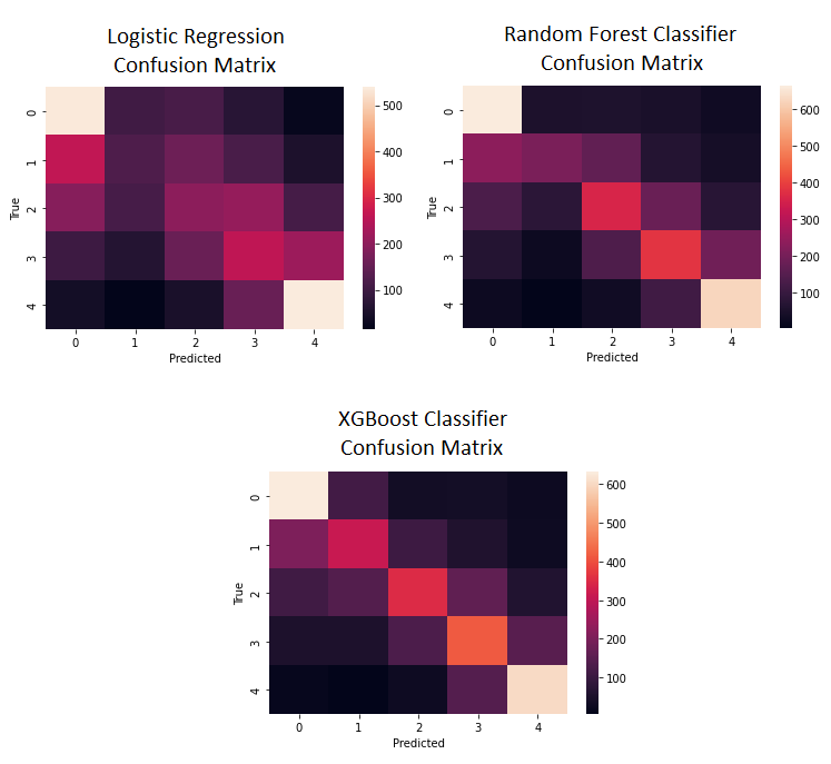
Among the optimized machine learning models, as predicted in previous section, XGBoost Classifier and XGBoost Regressor have better metric scores than Random Forest Classifier and their simpler counterparts.
2.4.1 Residual Diagnostics
The residual is the difference between the model predicted and the actual value of the dependent variable to quantify the quality of the predictions obtained from the model. In this section, to observe the performances of the regression models, the absolute values of residuals will be used. In order to obtain a “good model”, the absolute values of the residuals should be small and not systematic. Ideal residues should be “white noise”, meaning that they should not contain hidden information about the explained variable.
Plot 4. 300 Residuals

Plot 5. 10 000 Resiudals

As shown, the Ridge model compared to the machine-learning models has the highest values of absolute residuals. In general for 10000 analyzed residuals Random Forest Regressor has greater number of outliers than XGB Regressor for greater predicted income. Comparing XGB Regressor to the others, not only are the residuals generally smaller, but also do not show any significant trends based on the value of the predicted income. The XGB Regressor seems to be the most stable model for this type of data and will be used further.
2.5 Explanations
2.5.1 Local Interpretable Model-agnostic Explanations
Local Interpretable Model-agnostic Explanations (LIME) serves to understand the factors that influence a complex black-box model around a single observation. It is a technique that approximates any black-box model with a local, more interpretable model to explain each individual prediction. In this section for the regression, LIME shows the impact of different explanatory variables for the prediction between minimum (which is the starting position) and maximum income. As for the classification, the explanations will be shown for influence of explanatory variables on probability to be classified into the group with the lowest income.
The chosen observation for this analysis is client with overall features closest to median, and the compared XGB models type, Random Forest models type and Logistic Regression. The linear model is not shown, because that model is unexpected to give reasonable results for that type of explanation for the majority of observations.
Plot 6. LIME Regression XGBRegressor

For XGBRegressor and that specific observation variables related to income from salary had the greatest influence on increasing the predicted income. The six months’ total expenditure of the observation had the greatest negative impact on predicted income. The expenses on cleaning service from different time periods had a suppressing impact on predicted income.
Plot 7. LIME Regression Random Forest Regressor

For Random Forest Regressor and that specific observation, explanatory variable related to income from salary had the significant impact on predicted income. The six months total income of the observation similarly to XGBRegressr has negative impact on predicted income, as well as total amount of client’s income for remuneration in the last six months had the most significant positive impact on prediction. However unlike the XGBRegressor, the Random Forest Regressor takes into consideration the negative impact of observations expenses related to PKS transport, but that impact is suppressed by the share of those expenses in total expenses in the last full month, which is similar to the variables related to expenses on cleaning services in Random Forest Regressor LIME explanation.
Plot 8. LIME Classification XGBClassifier

Plot 9. LIME Classification Random Forest Classifier

Plot 10. LIME Classification Logistic Regression

The structure of LIME explanations for XGBClassifier look similar to those of Logistic Regression. Both of those models take into account some variables that are in favor of probability to be classified to group with the lowest income, whereas the explanation for Random Forest Classifier focuses mainly on variables that have negative income on that probability, except the amount of six months total expenses. For XGBClassifier and Random Forest Classifier, the client’s income from salary in different periods have significant negative impact on being classified to group with the lowest income, whereas Logistic Regression shows that the most significant impact on income have variables such as income for rental or expenses related to cleaning services.
In general, LIME explanations for XGBRegressor and Random Forest Regressor share some similarities for the explanations of their predicted income, but take different types of variable from the same category into account. As for the explanations for the classification, both XGBClassifier and Logistic Regression consider variables, that are in favor of being classified to the group with the lowest income, whereas Random Forest Classifier focuses on those who negatively affect that probability. It is worth mentioning that for the classification, the explanatory variables have the strongest negative/positive impact on probability for the Logistic Regression, then XGBClassifier and finally Random Forest Classifier with the strongest absolute impact being less than 0.03.
2.5.2 Ceteris Paribus Profiles
The Ceteris-paribus Profiles (CP) show how a model’s prediction would change if the value of a single explanatory variable changed. In this section, the Ceteris Paribus Profiles will be created for some of the most important variables for XGB model type (see section: Variable Importance). The observation for this analyzes is the client with overall features closest to median and the compared models are XGB type, Random Forest type and Logistic Regression. The linear model is not shown, because the predicted income for that observation is much higher than its actual value.
The analyzed explanatory variables:
- Six months total income
- Six months total expenditure
- Age
2.5.2.1 Six months total income
Plot 11. Six months total income Regression

The explanations of XGBRegressor are opposite to Random Forest Regressor, and are more consistent with intuition, that would suggest increase of current income if the prior six months income had enlarged. The XGBRegressor model suggests, that with all his other features unchanged, his predicted income will be greater only up to around 180 000 PLN of last six months total income.
Plot 12. Six months total income Classification XGBClassifier

Plot 13. Six months total income Classification Random Forest Classifier

Plot 14. Six months total income Classification Logistic Regression

The explanations for XGBClassifier indicate, that client is more likely to be qualified by that model to a group with greater income as his previous six months total income would increase. The results of Random Forest Classifier suggest a more “cautious” approach, where the probability of being qualified by the model to group with higher income is not changing as much as in XGBClassifier. Both models indicate, however, that the highest probability is still to be qualified to the first group with the lowest income regardless of the changes of that explanatory variable. Logistic Regressor does not show reasonable results.
2.5.2.2 Six months total expenditure
Plot 15. Six months total expenditure Regression

The Random Forest Regressor predicts greater changes in income with the increase of previous six months total expenditure than XGBRegressor. Given that the predicted income by XGBRegressor is closer to real value, it might strenghten the assumption that Random Forest Regressor might more often overestimate or undervalue predicted income than XGB Regressor (see section: Residual Diagnostics).
Plot 16. Six months total expenditure Classification XGBClassifier

Plot 17. Six months total expenditure Classification Random Forest Classifier

Plot 18. Six months total expenditure Classification Logistic Regression

The difference between Random Forest Classifier and XGBClassifier explanations is stronger than in previous classification. Random Forest Classifier suggest small changes in probability of being classified by the model to a group with greater income by changing previous six months total expenditure, however XGBClassifier results suggest that further increase of previous six months total expenditure after crossing the point of 60000 PLN strongly increases the probability of being qualified to the group with the highest income. Logistic Regression slightly lowers probability of being classified to group 4 with greater previous six months total expenditure”
2.5.2.3 Age
Plot 19. Six months total expenditure Regression

Surprisingly, the explanations for Random Forest Regressor indicate that for client with overall features closest to median the changes in his age have no impact on predicted income, which is not compatible with the hypothesis concluded in the Mincer Equation. The explanations of XGBRegressor however indicate according to Mincer Equation, that with greater age, greater income is expected, however it shows that the predicted income will not increase after age greater than 38. That point might be interpreted as the peak of someone’s career.
Plot 20. Age Classification XGBClassifier

Plot 21. Age Random Forest Classifier

Plot 22. Age Logistic Regression

The explanations of XGBClassifier indicate that with greater age, the probability of being classified by the model to the group with the lowest income significantly drops. After the age of 23, the highest probability is for that observation to be classified into the second income group. Random Forest Classifier shows little changes with most significant change in probabilities at the age of 28. The explanation of Logistic Regression does not imply any changes at all.
Those examples of Ceteris Paribus Profiles show, that XGB type of models have the most interesting explanations, which follow intuition for client with overall features closest to median. The Random Forest type of models in general are showing small changes in prediction with changes of the explanatory variable, which is similar to the LIME explanations for that model (see section: Local Interpretable Model-agnostic Explanations), whereas Logistic Regression suggest little to no changes in prediction at all.
2.5.3 SHAP
The following image presents SHAP summary plot for XGB Regressor and all observations from the dataset. The total amount of the customer’s expenses in the last 6 months appears to be the most important factor affecting model output, with a clear relationship - the more expenses, the greater positive impact on the estimated earnings. Overall, variables concerning remuneration and expenses seems to be the most important for the model.
Plot 23. SHAP summary
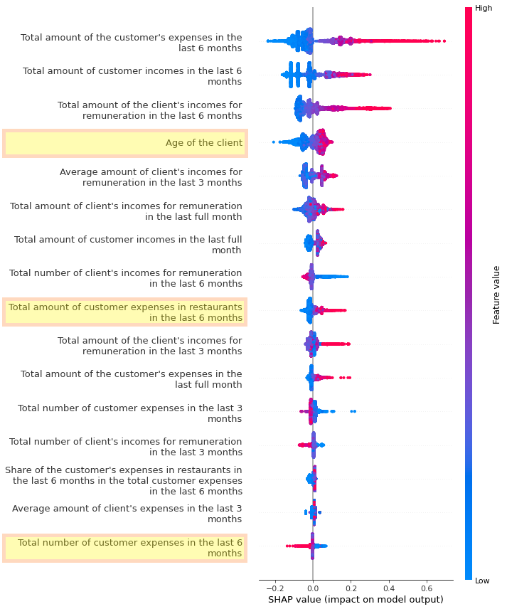
Other interesting variables were marked in yellow. The plot indicates that lower age has a negative impact on estimation results. Higher age generally increases predictions, but the relationship is not as clear as in the previous example - for some group of clients, medium age has a more positive impact on the earnings estimation than for older clients.
For the total amount of customers expenses in restaurants in the last 6 months and for the total number of customer expenses in the last 6 months, there are possible relationships between the highest values and model output. For the first variable there is a possibility that clients with the highest expenses of that type will have higher estimated earnings and the second one indicates a possibility that clients with higher number of expenses will have lower estimated earnings. However, there are not many clients with very high values of these variables and the possible relationships may be only artifacts. A continuation of the analysis of the mentioned variables is presented in the Partial Dependence Profiles section.
2.5.4 Partial Dependence Profiles
The Partial-dependence Profiles (PDP) are created by taking the mean of the Ceteris Paribus profiles for all observations. It shows the summary of how a change of single explanatory variable impacts model’s predictions (in general). In this section, XGB type of model will be compared with its simpler counterparts (Ridge and Logistic Regression).
The analyzed explanatory variables:
- Six months total income
- Six months total expenditure
- Three months total income
- Age
Plot 24. Partial-dependence Profiles Regression
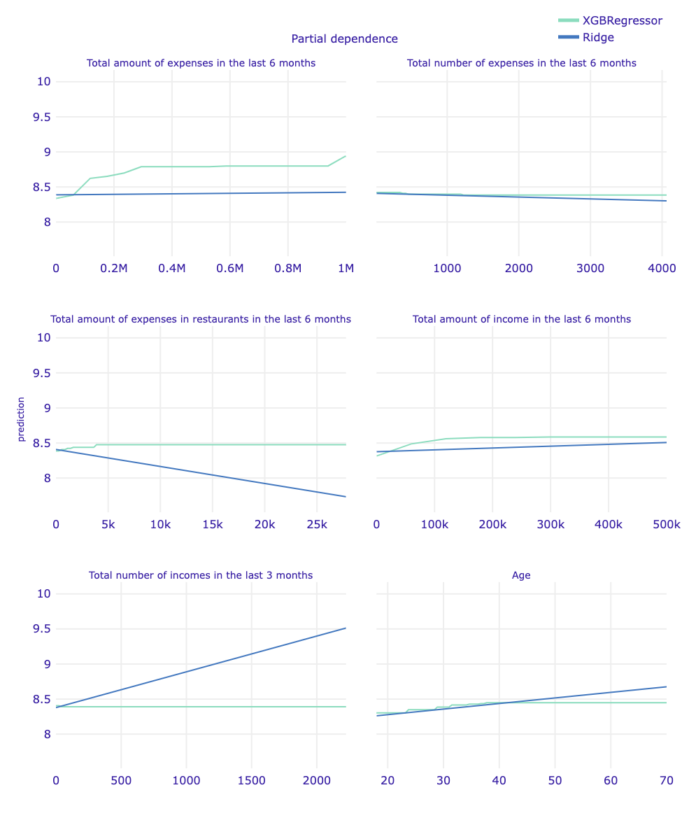
The PDP explanations for XGBRegressor show that both income and expenditure from the last six months are important, and their change increase the predicted income. XGBR also detects possible changes with six months expenditure greater than 900 000 PLN, which suggest that the model can identify clients with much higher income. Ridge PDP explanations suggest, that changes in the last three months are more important for the prediction of income than those in longer period, which is opposite to what the XGBRegressor model suggest. XGBRegressor PDP explanation for age is similar to that of the CP for client with features closest to median. Both Ridge and XGBRegressor globally confirm hypothesis in Mincer equation, however the linear model does not show the point, that can be assumed as “peak of the career” and assumes constant growth of predicted income even for client with age 65.
Plot 25. Partial-dependence Profiles XGBClassifier
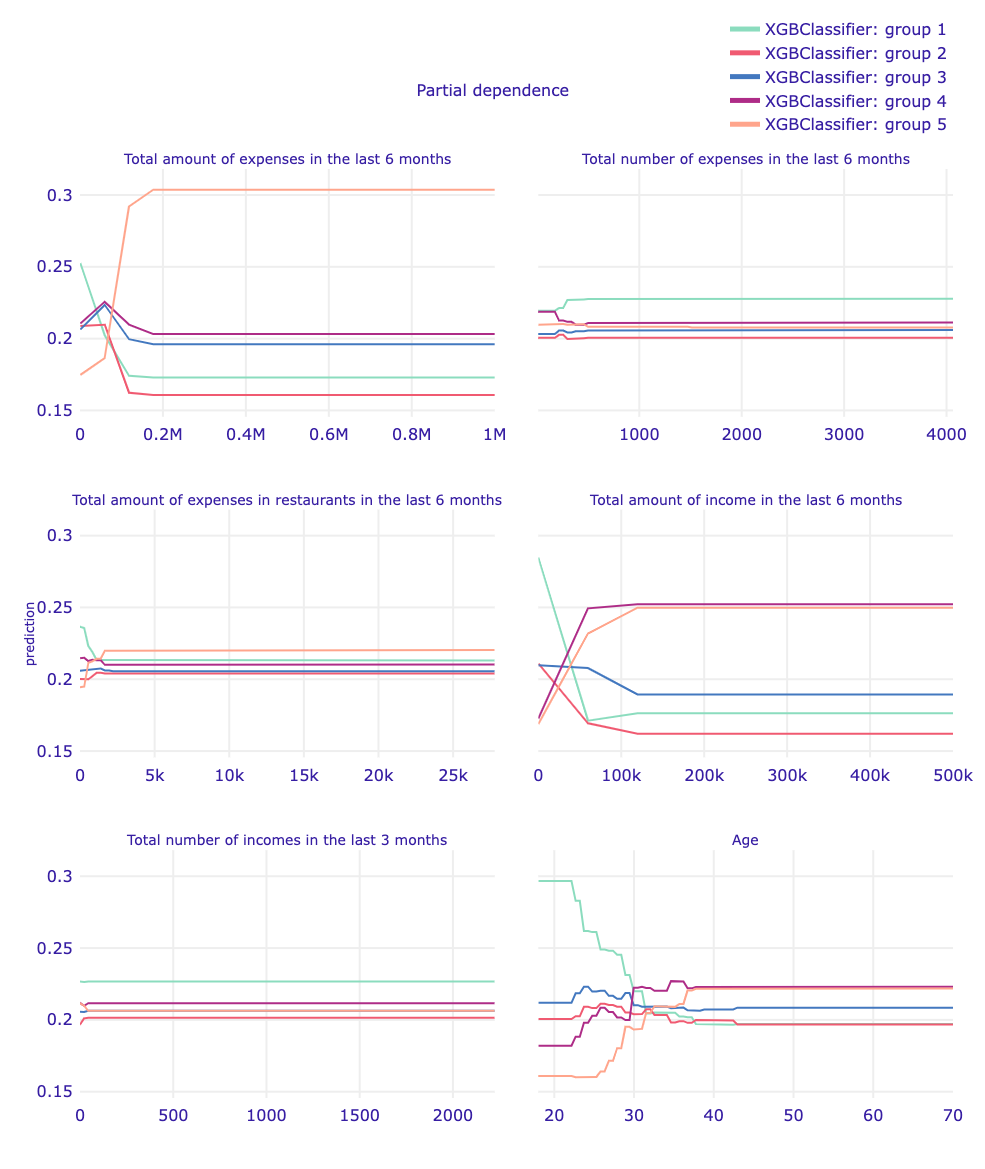
The XGBClassifier globally indicates that changes in six months total expenditure impact the highest probability for being classified to a group with either lowest, middle or highest income. Unlike for six months total expenditure, with the changes in six months total income greater 200 000 PLN does not come the highest probability for being classified to the group with the highest income. The global results however differ from the local CP Profile for client with overall features closest to median, where changes in six months total income did not mean that the probability of being qualified to the group with the lowest income ceased to be the highest. Changes in three months total income are not considered as important for this model, and the increasing probability of being classified to the group with greater income with greater age confirms the hypothesis in Mincer equation.
Plot 26. Partial-dependence Profiles Logistic Regression
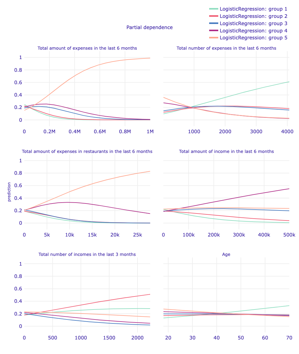
The explanation of six months total expenditure changes for Logistic Regression is similar to XGBClassifier. Changes in six months total income are similarly to XGBClassifier suggesting that after a certain point the highest probability is for being classified to group with second-highest income, however those changes in probability are for smaller amount of six months total income than in XGBClassifier model. The Logistic Regression also takes into consideration three months total income, however the results make little sense, as with three months total income greater than 500, the probability of being classified to the group with second-lowest income is highest. Logistic Regression PDP explanation for age is directly opposite to hypothesis in Mincer equation, as the highest probability for being classified to group with the greatest income is for lowest age and the highest probability for being classified to group with the lowest income is for age greater than 40. The explanation of six months total expenditure changes for Logistic Regression is similar to XGBClassifier. Changes in six months total income are similarly to XGBClassifier suggesting that after a certain point the highest probability is for being classified to group with second-highest income, however those changes in probability are for smaller amount of six months total income than in XGBClassifier model. The Logistic Regression also takes into consideration three months total income, however the results make little sense, as with three months total income greater than 500, the probability of being classified to the group with second-lowest income is highest. Logistic Regression PDP explanation for age is directly opposite to hypothesis in Mincer equation, as the highest probability for being classified to group with the greatest income is for lowest age and the highest probability for being classified to group with the lowest income is for age greater than 40.
The shown Partial-dependence Profiles suggest that the global explanations for XGB type of models might be better to use than its simpler counterparts. Both XGBRegressor and XGBClassifier suggest that the explanatory variables from greater time period are more important than those from shorter time period, whereas the Logistic Regression and especially Ridge suggest that explanatory variables are significant. However, the initial assumption might be that although changes from a shorter period are closer to the current situation, the long-term changes are more important, because they represent the overall situation of the client. The explanations of XGB type of models are closer to that intuition.
2.5.5 Variable importance
Variable importance is a measure of how much a given variable or set of variables is useful for the model to make most accurate predictions. In this section, we cover the variable importance analysis for XGBoost Regression, XGBoost Classifier, Logistic Regression and Ridge Regression models. For every asset A, we were provided with the following variables (with income/outcome based on the nature of A):
- One month total income/outcome for
A; - Three months total income/outcome for
A; - Six months total income/outcome for
A; - One month number of transactions for
A; - Three months number of transactions for
A; - Six months number of transactions for
A; - Average income/outcome for
A;
and exceptionally one variable for the age.
2.5.5.1 Grouped variables
During our work, we were interested in which assets our models value the most. We have created groups of explanatory variables by assets to perform importance analysis using dalex.
2.5.5.1.1 Ridge regression
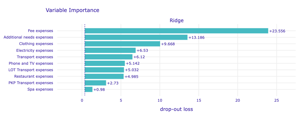
Ridge regression model finds variables related to general fee expenses definitely the most valuable for predictions. In addition, the model definitely values variables related to additional needs and clothing expenditure above all others. As we will see later, its opinion is unique across our 4 study models.
2.5.5.1.2 XGB regressor
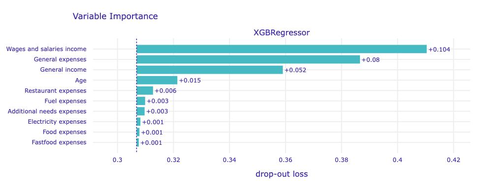
In this case, the model favorites its strict top 4 of variables related to respectively:
- Salaries income
- General expenses
- General income
- Age
putting most of its attention into salaries and general expenses.
2.5.5.1.3 Logistic regression
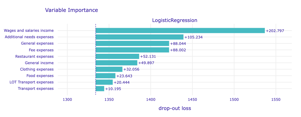
The Logistic regression model shares high interest for salaries and general expenses with XGB models, with the difference in cases of fee and additional needs expenses.
2.5.5.1.4 XGB classifier
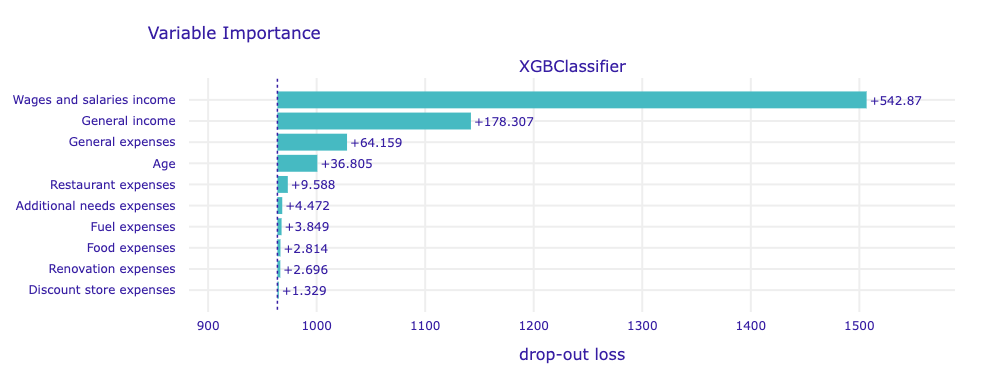
This model considers as the most relevant the very similar set of variables as its regression XGB brother, with the difference of paying much more attention to salaries income and rating general income much better than general expenses.
The latter 3 models, in addition to the seemingly obvious variables of general income, expenditure, and earnings, pay considerable attention to the utility of the age variable while predicting income, which coincides with Mincer’s equation predicting earnings primarily on the basis of age.
2.5.5.2 Time horizon
This study has been performed on variables grouped by time intervals (i.e. 1 month, 3 months and 6 months)


In this study, we do not notice any discrepancy in the importance ratings of the above models. Each strongly prefers to have a broader view of the temporal range of the data provided. The situation changes somewhat in the following case

where XGBoost classifier considers the longest variables to be the most important, and pays similar attention to those representing data from three months and one month, with a slight emphasis on the shorter ones.
2.6 Explanations validation
2.6.1 Survey description
In order to evaluate explanations of the models, there was conducted an internet survey. The idea was to show people explanations of models with different performance (best XGBoost models compared to simple Ridge and Logistic Regression). The hypothesis was that interviewees would be able to choose which models are better and would trust them more based on only the explanations. If it was true, then a statement could be posed that our best models give better explanations than the ones from simple models.
The survey consisted of 3 parts, each based on different types of explanations - SHAP model summary, Variable Importance, Partial Dependence Profiles for Age variable. Explanations were generated for the following models:
- Model 1 - Ridge regressor without hyperparameters optimization
- Model 2 - optimized XGBoost regressor
- Model 3 - Logistic Regression classifier without hyperparameters optimization
- Model 4 - optimized XGBoost classifier
The interviewees did not know architecture of any model and did not have any information about their performance. A numeric label and explanations were the only data. The survey was aimed at a group of people with some analytical thinking skills, but without specific knowledge from fields such as machine learning. There was a concern that showing plots with descriptions of methods and requiring their understanding could be a demanding and time-consuming task for the interviewees. Therefore, the graphical explanations were transformed to textual descriptions. They were also simplified in some cases, e.g. in the SHAP summary plot there were many similar variables with different time horizons, so the time horizon was omitted. Below there are translated explanations (the original survey was conducted in Polish language):
- SHAP model summary
- Model 1
- greater amount of client’s expenses on fees (electricity, rent, cleaning services) increases the income estimate
- less house spending increases the income estimate
- large expenses for additional needs (hobby, cinema, theater, restaurant) increase the income estimate
- Model 2
- a high amount of expenses increases the income estimate
- high age increases the income assessment
- a high amount of expenses in restaurants increases the income estimate
- a low NUMBER (number of transfers) of customer receipts increases the income estimate
- Model 3
- greater amount of client’s expenses on fees (electricity, rent, cleaning services) increases the income estimate
- less house spending increases the income estimate
- large expenses for additional needs (hobby, cinema, theater, restaurant) increase the income estimate
- Model 4
- a high amount of expenses increases the income estimate
- high age increases the income assessment
- a low NUMBER (number of transfers) of customer receipts increases the income estimate
- Variable Importance
- Model 1
- the sum of expenses on fees and the sum of expenses related to the house - the variables from these groups had the greatest impact on the result of the estimation
- variables from the next four groups, respectively: sum of expenses for additional needs, transport, clothes and air transport - also important for the model, but have a smaller impact
- Model 2
- the sum of the salary receipts, by far the most significant
- consecutively, the sum of expenses and sum of all receipts - less but still important for the model
- the age of the client of less than the above but still significant significance
- Model 3
- the sum of the salary receipts, by far the most significant
- consecutively, the sum of expenses for additional needs, sum of all expenses and sum of expenses for fees - less but still relevant to the model
- consecutively, the sum of expenses in restaurants, the sum of receipts and the sum of expenses for a house with a lower than above but still outstanding significance
- Model 4
- the sum of the salary receipts, by far the most significant
- sum of all receipts - less but still relevant to the model
- consecutively, the sum of expenses and the age of the client with a lower than above-mentioned but still significant significance
- Partial Dependence Profiles for Age
- Model 1 - as the age rises between 20 and 70, the estimated income grows at the same rate
- Model 2 - between the ages of 20 and 40, the estimated income grows at a similar rate, after the age of 40 stabilizes
- Model 3 - before the age of 45, the greater the chance that the model will estimate high income, after the age of 45, the greater the chance that it will estimate low income
- Model 4 - between the ages of 20 and 35, the chance of estimating low income by the model decreases and the chance of estimating high income increases. After 35 years of age, the model’s estimates stabilize, returning rather large incomes and less frequently quite small
After every part there was the same question:
Based on the partial explanation in the section above, how well can each model work? (1 - model estimates may differ significantly from actual income, 5 - model estimates may be very similar to actual income)
2.6.2 Survey results
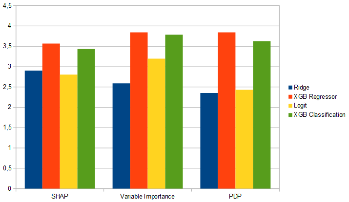
Below, there are the average ratings for each model in each section, collected from 51 answers. As the results show, better models scored better in each section. Especially for the PDP-based explanations, interviewees gave clearly higher rates for XGBoost models than for the simple ones. For SHAP-based explanations, the results are not as clear, but still the best models got better rates.
On the next image there are average results not splitted on different sections. XGBoost models got better results from the entire survey. This confirms the hypothesis posed in the description. Based on the results, people trust more explanations generated from the best XGBoost models and rate this models with 3.5 on average on 1-5 scale.
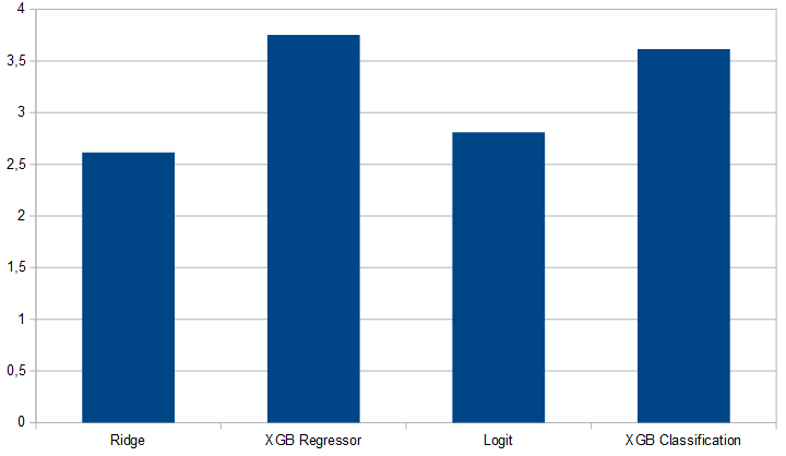
Explanations from XGBoost regression and classification were not the same, but similar. The regressor got a slightly better rating, but the difference between the classifier rating is too low to be statistically significant.
2.7 Summary and conclusions
The Random Forest Regressor does not confirm the hypothesis in Mincer equation, and the prediction is often overvalued. Random Forest Classifier has worse accuracy than XGBClassifier and the explanations show little changes in prediction by changing the value of explanatory variable
The overall analysis shows, that XGB type of models have better performances and both more interesting and closer to intuition results, therefore are recommended for analyzing this type of data. The results for XGBRegressor and XGBClassifier are equally satisfying, which is why they are both equally proposed and can be used depending on the situation.
As shown by the explanations of the best-performing XGBoost models, the variables concerning remuneration and total expenses were the most important for the results of the estimation. The impact of the information on the expenditure target was rather marginal. For the best models, only in some cases these variables were meaningful.
In addition to the remuneration and expenses variables, age also turned out to be quite an important factor influencing estimated earnings. This variable is correlated with work experience, which is consistent with the Mincer equation.