Chapter 1 Predicting loan applications
*Authors: Krzysztof Bober, Jan Ciołek, Jakub Dylik, Michał Niedziółka, Anna Stykowska
*Mentors: Amadeusz Andrzejewski, Kaja Grzywaczewska, Rafał Walasek, Mateusz Zawisza
1.1 Introduction
1.1.1 The problem
Our team’s task was to find essential factors, affecting the number of loans granted by one of the major Polish banks, by building the so-called propensity to buy model.
Research was based on client’s transaction history which included variation of average economic behaviour represented by microdata. Using shared data our team’s main goal was to emerge a typical customer who has applied for a loan (dependent variable: 0- client haven’t applied for a loan, 1- client have applied for a loan). Described by dependent variables type of average bank’s customer leads to more precise matching banking, and as a result maximalize profits.
1.1.2 The data
Client’s transaction history is build with 392 dependent variables divided into 7 categories:
- total amount of expenses/ income during the last month,
- total amount of expenses/ income during the last three months,
- total amount of expenses/ income during the last six months,
- average amount of expenses/ income in the last three months,
- total number of expenses/ income during the last month,
- total number of expenses/ income during the last three months,
- total number of expenses/ income during the last six months.
The data concerns both basic transactions, as fees or salary, as well as less popular types of transactions, such as expenses/ income from alimony or expenses for various types of charities.
Besides original microdata, in the database can be found a set of variables created by adding up or dividing similar groups of factors in different time intervals.
The research conducted was based on 10.000 records. According to the sample size it is reasonable to expect representativeness therefore could lead to obtaining real factors affecting the number of loans granted by the bank.
1.2 Preparing the data
1.2.1 Data preprocessing
The first step for entering the data into the model was to check the correlation between individual features (columns in our database). We decided that we will reject variables that are correlated with each other by more than 0.8. We found that the explained variable was not significantly related to any of the explanatory variables.
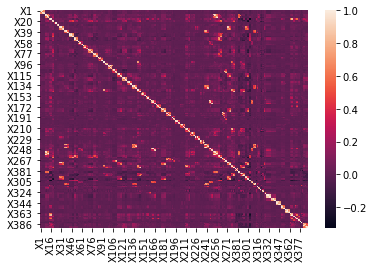
As we can see, the most correlated variables are on the main diagonal. This is due to the fact that the data was divided into specific income and expense groups and then time intervals (1 month, 3 months and 6 months) were specified, which gave several variables that could be very dependent on each other.
1.2.2 Forward selection
After the operation of removing over correlated variables, it was possible to reduce the number of variables by more than a half, but there were still too many of them to enter all of them into the final model. When trying to associate different variables with each other or transform them (using a logarithm, squaring, etc.) We did not find a significant linear relationship. similar transformations could adversely affect the model’s explainability so we decided to use the forward selection algorithm to select the best variables. This type of stepwise selection allows us to select the most important explanatory variables by entering successive predictors into the model until certain conditions are met (adequate accuracy with a small number of variables - in our case 16).
In the first step, the regression model is fitted with the intercept only, without predictors. The value of the chosen metric (AUC/gini) is calculated with the aim to test the correctness of the regression model constructed in this way. Then the algorithm adds sequentially one predictor which allows to obtain the best result.
1.3 Models
1.3.1 Choosing the model
We tested a variety of different approaches to this problem. Evaluation was done using balanced accuracy and AUC ROC metrics. For every model we did the same steps: data preprocessing, training, evaluation on validation set. We were also tuning hyperparameters, but we won’t mention them for models that were only experiments and weren’t used in the final model.
1.3.2 Metrics
Accuracy

where TP = True positive; FP = False positive; TN = True negative; FN = False negative. In our case, it’s not the best metric, because our data is not balanced – around 80% negative
Balanced Accuracy
\(Sensitivity = \frac{TP}{TP + FN}\)
\(Specifity = \frac{TN}{TN + FP}\)
Balanced accuracy is a mean of sensitivity and specificity. It solves our problem of unbalanced classes. Below you’ll see this metric quite often.
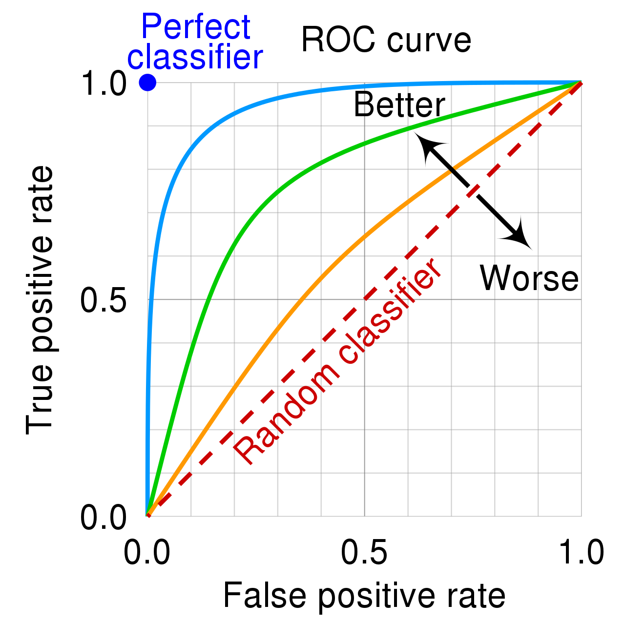
AUC ROC
A receiver operating characteristic curve, or ROC curve illustrates the diagnostic ability of a binary classifier system. The ROC curve is created by plotting the true positive rate (TPR) against the false positive rate (FPR) at various threshold settings (they were named in balanced accuracy as Sensitivity and Specificity). AUC stands for area under the curve, and in our case the closer it gets to 1 the better.
1.3.3 Linear models
We tested two important models, linear regression and ridge regression. We started from standard linear regression with data normalized to [0, 1] range. Model achieved:
Linear regression
| Metric | Train | Validation |
|---|---|---|
| Balanced Accuracy | 0.831 | 0.512 |
| AUC | 0.761 | 0.672 |
Significant overfitting can be seen, let’s try to add regularization. We’ll use Ridge Regression for this. To the function that should be minimized, we’ll add a new sum, which will penalize the model for trusting a single parameter too much.

Ridge regression
| Metric | Train | Validation |
|---|---|---|
| Balanced Accuracy | 0.828 | 0.512 |
| AUC | 0.746 | 0.690 |
1.3.4 TabNet
TabNet uses sequential attention to choose which features to reason from at each decision step, enabling interpretability and more efficient learning as the learning capacity is used for the most salient features. In this picture, you can see a general idea for processing the tabular data by TabNet.

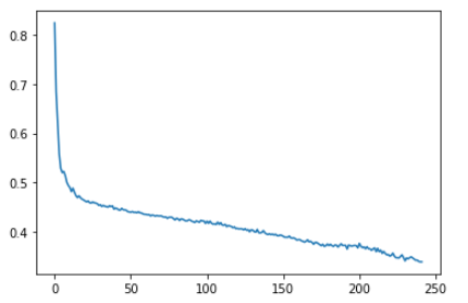
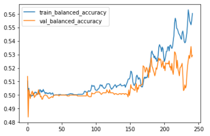
We trained the model on different hyperparameters, the most promising were the default ones. These are learning curve and balanced accuracies charts.
TabNet
| Metric | Train | Validation |
|---|---|---|
| Balanced Accuracy | 0.56 | 0.529 |
| AUC | 0.745 | 0.596 |
Unfortunately, TabNet results aren’t enough
1.3.5 Trees
We tried a few popular models:
- Random forest
- XGBoost
- CatBoost
- Light GBM
In the end we chose LGBM as it produced the best results.
Light GBM (Light Gradient Boosting Machine) is a machine learning model based on decision trees that uses gradient boosting in classification and regression tasks. Light GBM improves the values of leaves not at the tree level – as most similar algorithms do – but already at the leaf level. This should result in the greatest loss reduction.
For this purpose, Light GBM uses histogram-based algorithms
that arrange the feature values into discrete groups.
This solution is faster than an attempt to choose the best split point for the leaf,
but we must control overfitting, among others, by keeping the parameter of the maximum tree depth under control.
With the aim to verify the correctness of the model,
we divided the data into two subsets: the test set and the training set in the proportion of 7: 3.
In order to select the appropriate parameters for training of the light GBM model,
we used the built-in GridSearchCV function. This function allows us to choose the best options for
given parameters from the vectors of values by calculating each time the selected accuracy metric for the model (AUC).
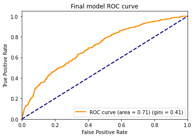
Using LGBM we have achieved a ROC AUC score of 0.71.
1.4 Explanations
Once the LightGBM model was trained and ready, it was time to start explaining its decisions. To explain our model we made use of many methods, including:
- Variable importance
- Partial dependency profiles
- Ceteris paribus
- Shapley values
- Break down
- LIME
Below we present the key takeways:
1.4.1 Variable importance
We started out by looking at the importance of all 16 of the chosen variables.
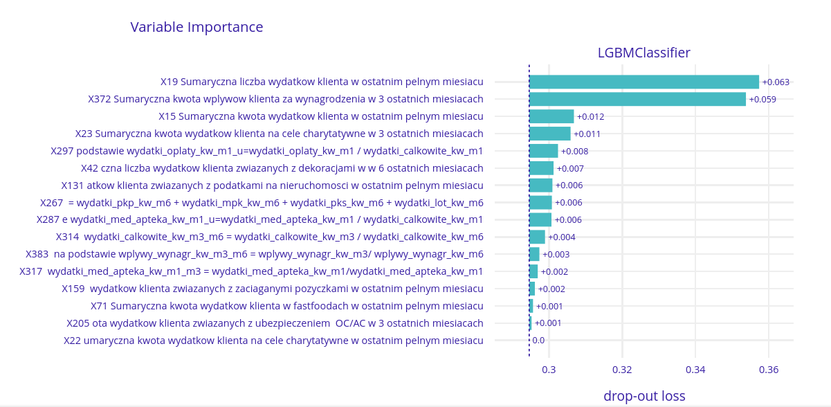
It’s clearly visible that there are two variables with the most importance. Those variables are:
- X19 - Total number of expenses in the last month
- X372 - Total income from the last three months
These results seem to be logical. Number and total amount of salary and expenses are the most intuitive variables affecting the willingness to submit a loan application.
1.4.2 Partial dependence profiles
Partial dependence profles allow us to see how various vales of a variable affect the prediction on average. Let’s take a look at four most important variables and see how their value influences the outcome.
The most important variable - X19 - Number of expenses in the last month
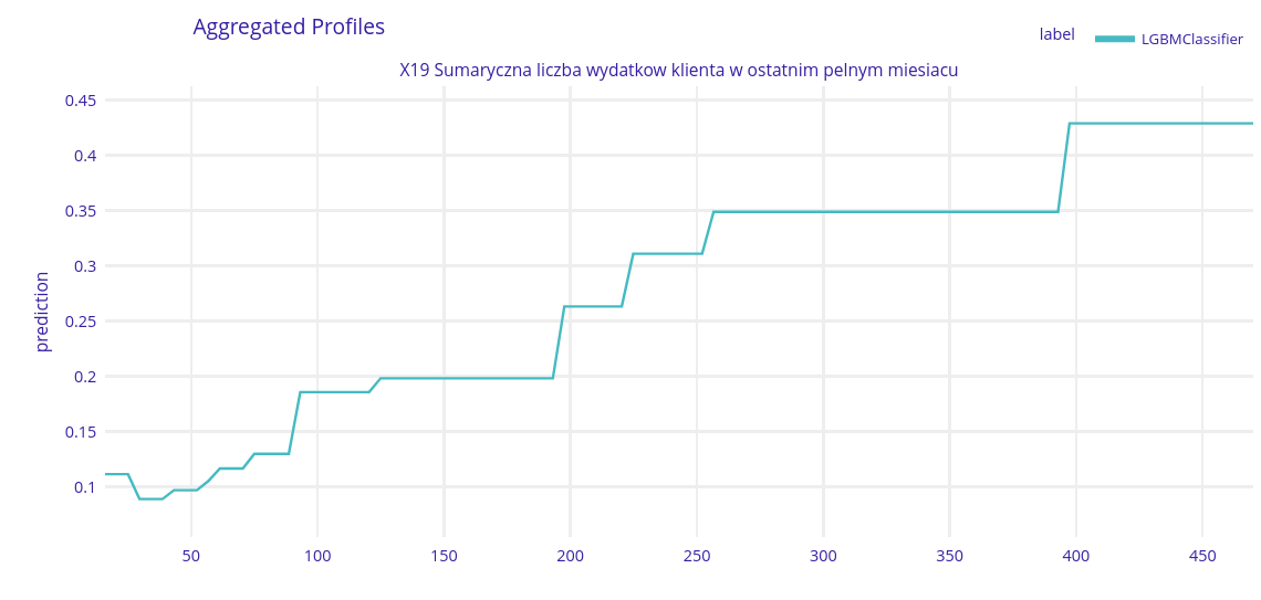
As the chart shows the more expenses someone has the more likely they are to request a loan. This makes sense - more expenses means that someone might be running out money and be in need of some help.
It’s internesting that the model chose the number of expenses and not the sum of their monetary value as the most important variable. It seems like the sum would be more important, but maybe there is more to it that meets the eye.
Second most important variable - X372 - Total income in the last three months
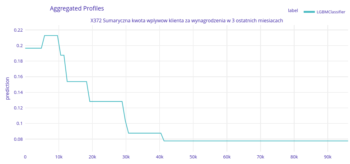
Here we can see that the less someone earns the more likely they are to apply for a loan. This is in line with the previous observation that loans are taken by people who have too many expenses.
If client earns more than 10 000 PLN by 3 last months the probability of taking the loan decreases regularly. What is more, we can split some groups of the clients (lack of trend changes) and if the total salary amount is bigger, the bigger the group is. After about 42 000 PLN threshold probability stays at 0.07 level.
Third most important variable - X15 - Sum of all expenses in the last month
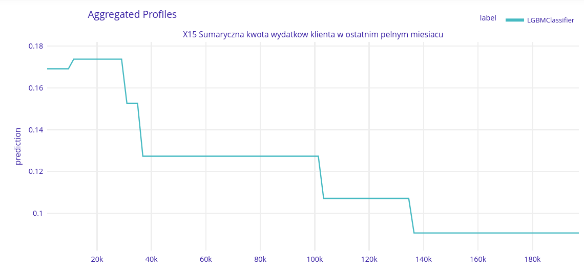
Despite having the number of expenses as the most important variable the model still chose their sum as the thrid variable. This might allow it to distinguish cases of many small expenses with higher accuracy.
Fourth most imporant variable - X23 - Sum of expenses for charity in the last three months
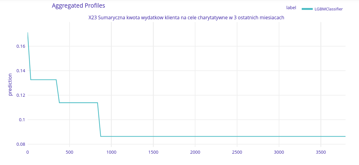
This one seems to be obvious. Main expenses for clients with smaller earnings are really basic (like rent, food, daily life costs), so they have no money for that purpose. Wealthier clients can afford donating the charity. If the client spent more than about 1000 PLN for the charity in the last 3 month, there is a really small Chance to submit a loan application.
1.4.3 Break down
Now let’s look at three samples with high, medium and low probability of taking a loan and trace the decision making process for them.
High probability client
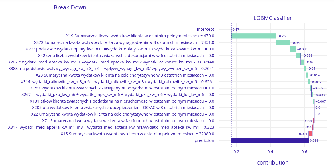
One more time, there are two crucial variables. X19 (total number of the client’s expenses last month) and X372 (total client’s salary last 3 months). This value is correlated with bigger chances of needing the loan.
Medium probability client
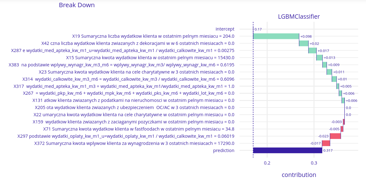
This chart shows again, that the importance of the X19 variable is one of the highest in this model. Contribution value here is higher by about a half than the second one – X42 (amount of client spending for decorations). The interesting fact is, another important variable – X372 has a negative contribution value here.
Low probability client
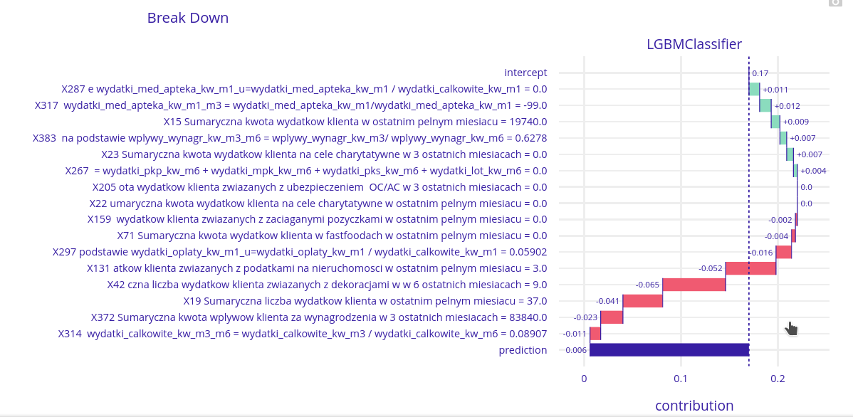
For a low probability client the situation is more interesting. X19 (total number of the client’s expenses last month) still has some influence (negative this time), but there are two variables that have a greater influence here:
X131 - Real estate taxes - This client had three expenses for real estate taxes in the last month. A person that owns three properties is likely wealthy and isn’t in need of a loan.
X42 - Expenses for decorations - people that can splurge on decorations probably have enough money to get by and don’t need a loan.
1.4.4 Profile of a typical loan taker
By analyzing the provided data we vere able to create a profile of the typical person that wants to apply for a loan. In the last month this person:
- Earned 4100 zł
- Had more than 900 expenses
- Spent more than 14 000zł (!)
- Didn’t really spend anything on decorations or charity
We were surprised how much this person spends - over three times the income. It might be that this person had a sudden large expense - a new car, health problems or some sudden repairs. They might not have enough money in the bank to cover that so they are forced to take out a loan.
1.5 Bussiness value
A bank could use this model to predict whether a given client is likely to apply for a loan or not. This knowledge could be used to optimize loan offering by targeting individuals likely to need a loan.
The bank has provided us with a gain matrix that can be used as a metric to judge how much value our model provides.
| true - 0 | true - 1 | |
| predicted - 0 | +2% | -5% |
| predicted - 1 | -2% | +5% |
This matrix rewards good predictions and penalizes wrong ones depending on severity of the mistake. In case where we predicted that someone wouldn’t apply for a loan but they did the penality is quite severe - each loan generates large profit for the bank. It’s better to be a little aggressive in the marketing and make sure that we don’t miss any clients that could possibly take a loan.
On the other hand the marketing can’t be too aggressive. Clients might get annoyed by constant spam of messages with various propositions. That’s why cases where the model wrongly predicted that a client would apply for a loan are also penalized, but to a lesser degree.
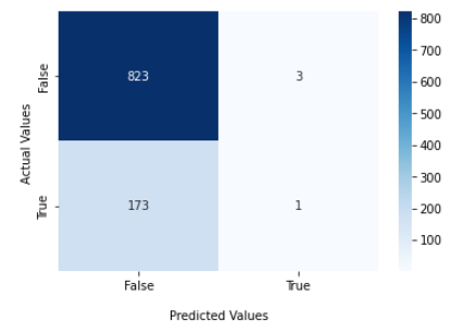
By choosing the right threshold above which the value is 1 we have achieved a gain of 1.007% per sample.
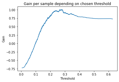
Thus according to this metric our model has tangible bussiness value.
1.6 Summary
During the project we have been presented with an interesting problem of finding out how likely a client is to apply for a loan. We analyzed the problem and prepared a model that is able to predict this likeliness with a decent accuracy. Then we used various explainable machine learning methods to figure out what the model considers as important and why does it make the decisions that it does. Finally we used a special metric to estimate profits that our model could provide to the bank and found out that it has real tangible business value.
Completing this project allowed us to learn many interesting facts about people that take loans. We have created a profile of the typical loan-taker and found a few aspects of it quite surprising.
By looking at model explainations we were able to figure out the major factors that decide whether someone would be likely to apply for a loan. Without explainable machine learning methods we would be in the dark as to how the model thinks, but thanks to them we were able to watch and learn what is really important.