Chapter 4 Selecting Clients of Bank that may want to apply for a loan.
Authors: Piotr Sotniczuk (University of Warsaw), Bartłomiej Gryglak (University of Łódź), Aleksandra Grzelik (University of Łódź)
Mentors: Karol Skorulski (McKinsey), Michał Szlupowicz (McKinsey), Michał Pyka (McKinsey)
4.1 Introduction
Bank loans, as popular as they are, prop up the bank sector. Consumption loans which accounted for the 15,44% of the credit in Poland in 2021* are the object of this chapters’ reflexion. The face value of the credit for consumption in Poland in 2021 reached 177,8 million PLN , which was lowered by the influence of covid crisis. Consumption loans, constituting an important part of the banks deposit , are as important assets for the commercial banks. It is also the case for mBank which is the partner of the Data Science in Practice project conducted by McKinsey & Company. Prediction of the customer’s propensity to buy enables the bank to optimize their advertisement strategy. Predicting that the client wants to apply for a loan, even before him knowing it, can shoot up the banks’ profits by targeting the groups willing to take a loan and optimizing the advertisement spendings. Knowing how precious is the information obtained via predictive models, we will pass to the overview of the analysis. The aim of the project is to create the best machine learning model, which will enable the bank to predict the propensity of appling for the loan of each client. This will make their advertisment proccess much better. Our goal is to firstly build a working model, then explain it and then validate whether our explanations are correct. This book is a report of our work.
*UKNF: Dane miesięczne sektora bankowego według stanu na 31 stycznia 2021 r.; Opracowano na bazie danych sprawozdawczych NBP z dnia: 01 marca 2021 r.
4.2 Model
Our goal was to build a model to classify whether or not a given customer would apply for credit.
4.2.1 Data:
We were given data that contained 393 columns and 1000 records. Each attribute occurred in three time periods: month, quarter, half year. The data contains only numeric values and there are no missing data.
4.2.2 Preprocessing
The first big obstacle was data imbalance.
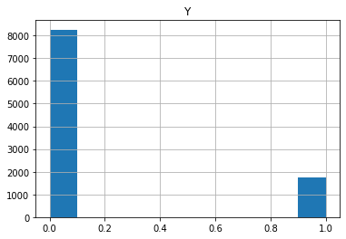
Due to the unbalanced nature of the dataset (only 17% of the data was comprised of customers who applied for credit), our first attempts at building the model gave unsatisfying results. Therefore, we used oversampling methods and took advantage of RandomOverSampler from the imbalanced-learn library. Thanks to this we have already obtained quite good results.
4.2.3 Model selection
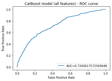
We expected the best results for methods based on gradient boosting since we were dealing with typical tabular data. We also tested models such as logistic regression, decision trees, SVM, k-nearest neighbour. As expected, the best results were obtained for gradient boosting. The open-source library Catboost worked best for us. In addition, we also used a logistic regression model for comparison, and it is easy to interpret due to its structure.
4.2.4 Selecting features
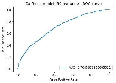
Because of the very large number of attributes, we decided to reduce it. We chose the n most significant variables. For n = 30 we obtained similar results to the model on full data. We selected the attributes that returned the highest feature importance values from the catboost model.
4.2.5 Using thresholds
Additionally, we checked how our model behaves when we select only a certain percentage of the best results where we have the highest probability that the customer will apply for a loan. This allows the bank to send notifications only to people who have a very high probability of applying for a loan. This could help a lot because usually there is a limited number of workers at call-center and it is impossible to call everybody, we need to choose most probable clients.
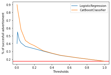
For example, if we select the top 10% of clients, 45% of them should apply for credit. If we want to call 1% of most probable clients about 90% of them will apply for a loan.
4.3 Explanations
We were using explanations for two types of receivers. First receiver is a person who wants to know if the model is working correctly, this could be a developer, a preson who wants to buy or use the model. This person should have at least basic knowledge in this area. Second type of receiver is a client of a bank who doesn’t have any knowlegde in this area. For this person it maybe interesting to know why for example he was targeted with advertisement.
Most of explanations were done on two models. Firstly did them on our model ‘Catboost’ and then on ‘Logistic Regression’ to have some perspective.
4.3.1 Feature Importance
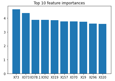
We looked at most important features in ‘Catboost’ API.
Then we used ‘Permutation Importance’ on both ‘Catboost’
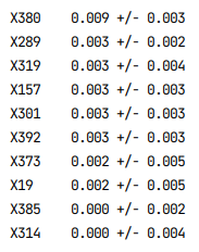
and ‘LR’ model to validate.
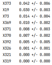
Features like ‘X373’, ‘X392’, ‘X73’, ‘X19’ were usually high in ranking so we knew that they are important.
4.3.2 SHAP Beeswarm
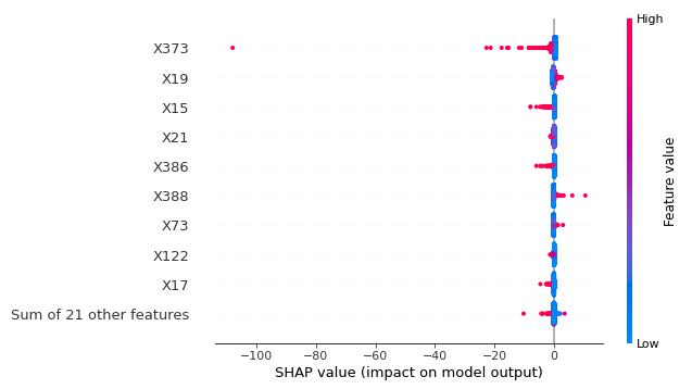
Now lets look into trends, we stared with very easy and usefull tool beeswarm plot.
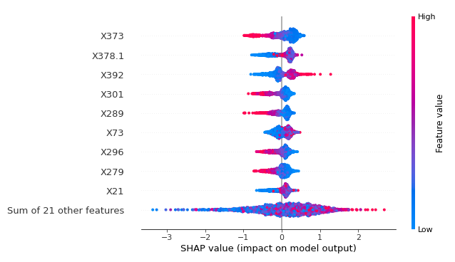
This plot shows how values of given feature affect the result. Red dots on the left in ‘X373’ (income for last 6 months says that high value of this feature decreases the possibility to apply for loan.
And for ‘LR’
4.3.3 PDP
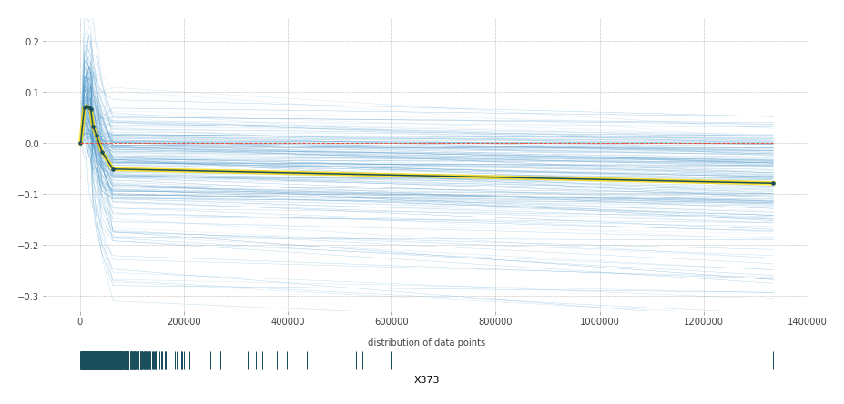
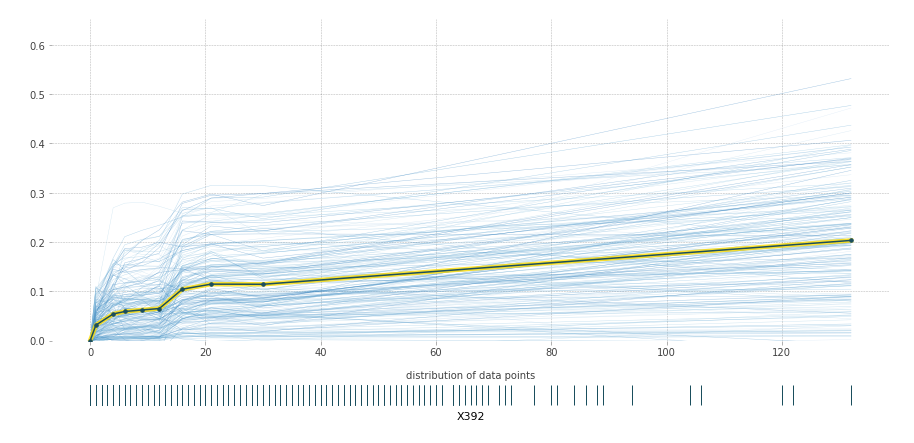
For most important and interesting features we also did PDP plots. Those plots show how the probability changes when we change the value of given feature for given client.
‘CatBoost’
And now for ‘LR’
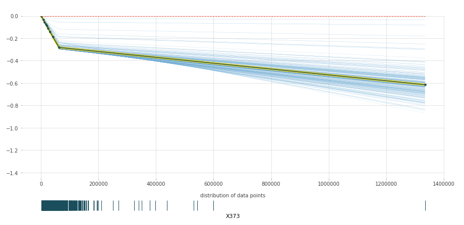
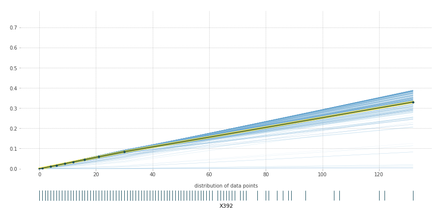
Plots from ‘LR’ are very simple (linear) but they keep the same trend as plots from ‘CatBoost’. This means the validation is positive.
4.3.4 Individual
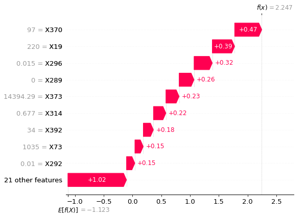
We also wanted to look into some individual explanations for the clients. Plots for clients that has a high or low score weren’t interesting. For breakdown plot all fetures were positive or negative with same impact on score like below.
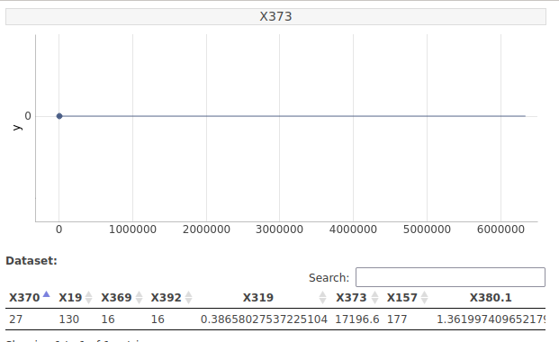
For Ceteris Paribus changing value was not affecting the score, it was a horizontal line like below.
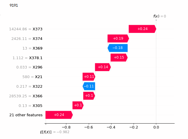
We plotted clients that were hard for model to classify, they were a bit more interesting but we didn’t went much deeper into this direction.
4.3.4.1 Breakdown
Breakdown plot shows most important features for given client and how they affect the result.
4.3.4.2 Ceteris Paribus
Ceteris Paribus shows how the score changes when value of given feature changes.

This plot is strange because it looks like the values jump from 0 to 1, this requires some more investigation. This direction wasn’t critical to the rest of the project so we left it. Both of the plots above weren’t really usefull for us at the moment.
4.3.5 Conclusions
After all this explanations we wanted to extract some bullet points that are most important. We also tried to think of reasons why given feature affects the score in this way. Score means probability of appling for loan by the client.
(X373) Higher income increases score, but only until a moment and then lowers score.
(X378, X380) If a person has a bigger income than outcome, then has a lower score.
(X296, X279) If someone spends high part of his income on pleasures, it lowers the score. (All of the points above shows that if a person has a lot of money, then he won’t need a loan.)
(X301) High NUMBER of bills transactions (water, electricity …) decreases the score. (If someone has many apartments, then he is wealthy and doesn’t need a loan.)
(X392) High NUMBER of transactions with ATM increases the score. (If someone needs to visit ATM often, then he lacks financial liquidity and probably needs some extra cash.)
(X73) High spendings in fastfoods increases the score. (This is a bit weird, but maybe wealthy people goes to fancy restaurants, poor people cooks food at home and the people in between eats in fastfood restaurants and those are our target grup.)
4.4 Validations
Now we wanted to check if our conclusions were right. We did this on many fields. We tried to validate them both on proffesionals and normal people (clients).
4.4.1 Mentors
First of all we talked with our mentors about our results. They helped us determine which conclusions could be a bug in data/model a what can be correct.
4.4.2 Second meeting
Thanks to the second presentation meeting we were able to talk to specialists also from the bank to get some feedback on both our work and results. They told us whether our conclusions match with their experience*. During the presentation we were also able to see work of other groups some of them had different topics of work but they still worked on similar data and that gave us some perspective.
*Interesting fact, at first X392-‘High Number of ATM transactions’ seemed to be very strange and looked like a bug in our model, but after the talk it turned out that this is very important feature and it really has a big impact on this problem.
4.4.3 We compared them to the report of ‘National Register of Debtors’ (KDR).
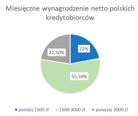
As it turns out our conclusion about the income of a client taking a loan was perfectly matching the report. People who earn a lot or not at all don’t take loans. It is the middle class.
4.4.4 Survey
We made a survey to ask ussual people what they think of our conclusions and how our explanations help them understand them. Firstly person had to learn how to read PDP and SHAP-Beeswarm plot and what information he can get from them. After this he was shown one conclusion with both Beeswarm and PDP plot and had to determine from 1-5 how much he agrees with it. Next we asked which plot shows this conclusion better.
It turns out most of the people agreed with conclusions (63% mean) and picked a PDP plot (28 to 16 votes). We may say that this information is usefull but we have some doubts about the results. People tend to agree to given statements (or in our case conclusions) and the PDP plot was first to show so it may have influenced the results.
PDP vs SHAP-Beeswarm
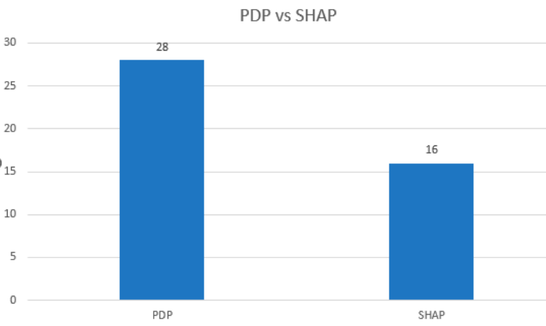
We testes points 1, 3, 4, 5 from conclusions above. Majority of answers for 1, 3, 5 conclusions where 4 or 5 (people agree with conclusion) and the PDP was choosen as better plot.
4.4.4.1 Conclusion 1
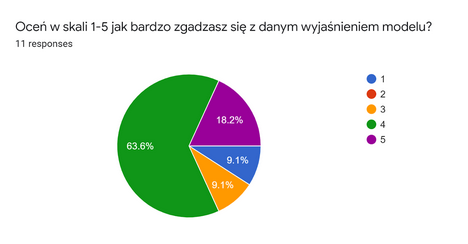
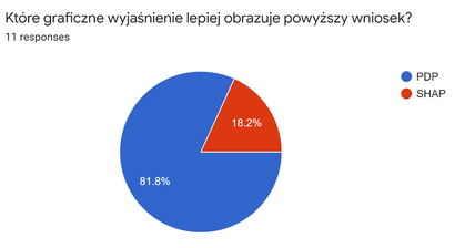
Results for conclusion 1. ‘(X373) Higher income increases score, but only until a moment and then lowers score.’
Agreement
Plots
4.4.4.2 Conclusion 4
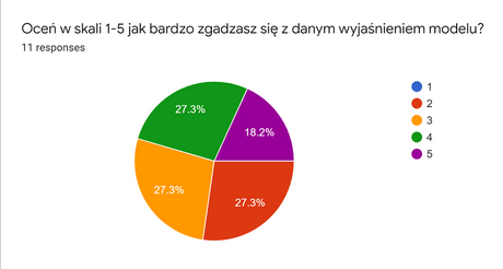
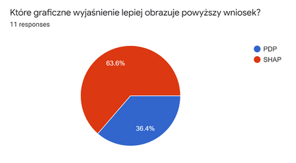
For conclusion 4. ‘(X301) High NUMBER of bills transactions (water, electricity …) decreases the score.’ it was different, people disagreed with this conclusion and SHAP-Beeswarm plot was better.
Agreement
Plots
4.5 Summary and conclusions
The final model turned out to be quite useful. Thanks to the threshold method the bank will be able to choose the clients with the highest propensity to take a loan, which could result in considerable profits. Only on the sample of 10 000 clients the catboost model can earn up to 240 000 PLN (the value on the 20% threshold). So depending on the threshold chosen (form 0,05, 0,1, 0,2) the models value stays in the range from 107 500 PLN to 240 000 PLN. The conclusions of the research are:
- High income reduces the likelihood of taking a loan.
- The probability of taking a loan decreases for the client whose earnings exceed the expenses.
- The greater the share of the income is spent on entertainment, the lower the likelihood of taking a loan.
- A large number of fees (electricity, rent, subscription, cleaning) reduces the likelihood of taking a loan.
- A large number of ATM transactions increases the probability of taking a loan.
- High expenses in fast food restaurants increase the likelihood of taking a loan.
The conclusions of the model seem to be logically correct. They were verified with publication of the National Debtors Register on the profile of the Polish borrower and judged by the respondents of public opinion poll, both with the satisfying outcome, which proves the conformity of the conclusions to both of the resources used.