Chapter 6 Why you won’t pay your loan back

Authors: Adriana Bukała, Zuzanna Kwiatkowska, Krzysztof Olejnik ¹ (University of Warsaw), Hubert Kacprzak, Bartłomiej Michalak, Barbara Wolska (University of Łódź)

Mentors: Michał Kaftanowicz, Andrzej Daniluk, Krzysztof Rewers (McKinsey & Company)

¹ A. Bukała, Z. Kwiatkowska and K. Olejnik contributed equally to all parts of the project. We also thank H. Kacprzak, B. Michalak and B. Wolska for their contribution to the feature engineering module.

6.1 Executive summary

• Our goal was to verify the possibility of automating default prediction by a machine learning model. Default is the situation in which a client stops paying the loan back to the bank.
• We decided to use the bank’s average profit on a single loan as our model selection metric. Our final model, Multi-Layered Perceptron, obtained an average profit of 334 PLN (69% of maximum profit) compared to the random model raising 266 PLN (55% of maximum profit).
• Based on the model’s explanations and the fact that it highly focuses on pharmacy expenses, we hypothesise that our model may have problems with fairness (with respect to health and gender), which must be fixed before using it in production.
• After explanations’ verification with potential users of the model, we observed that users prefer to see approximately 4 explanations on being denied a loan before they feel the information overload.

6.2 Introduction

Imagine a young girl, Catherine, age 25, who has just left college and started her first job as a software developer. She’s earning 3000 USD monthly, spending around 50 USD in discount stores, 100 USD on clothes and 500 USD in restaurants.

Would you give Catherine a small, 1000 USD loan for a new phone?

You may think - her situation looks fine. Or maybe you can’t make the choice based only on the information given.

But what if we told you, that amongst those few features there’s already one which guarantees us that Catherine won’t pay her loan back? Would it be true or would you find one based on your own biases?

No matter the answer, this short story introduces us to so-called default, ie. the situation in which a client stops paying their loan back to the bank. Increased default rate may result in unnecessary losses for the bank, while properly filtering out such clients can increase bank’s profit.

In order to avoid defaulting clients, credit officers thoroughly investigate prospects’ income sources and expenses. Such a process may be long and tedious but, due to the fact that it is a very isolated and well-defined task, it is in theory automatable by a machine learning system (which is also proven by existing tools in this area). An automation like this can be not only beneficial for the bank, to help their credit officers in making the right decisions, but also make the process of giving the loan faster and smoother for the client.

In this project, thanks to the data provided by one of the large Polish banks, we had the opportunity to explore:

1. is predicting default based on income and expenses possible using a machine learning system?
2. what factors, according to the model, contribute the most to a client defaulting on the loan?
3. are we able to distinguish between random and correct explanations justifying loan rejection when the number of information increases?

From the Data Scientist stance, our work involved exploring the data, creating the model and defining business metrics to validate it, exploring the model through explainability lenses and creating a survey to validate their quality. Such order and process is also preserved in the structure of the following report.

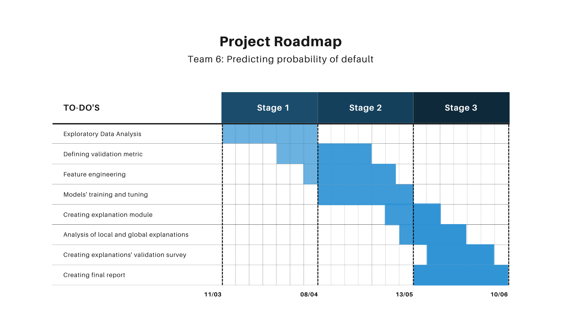
FIGURE 6.1: Project roadmap.

6.3 Data

The data represented a sample of young people (age 18-25) and described their expenses and sources of income in different categories. Before the project, it was anonymised by synthesising clients’ most typical financial profiles from the actual database of the bank’s clients. For each client, the data represented aggregations from the time period of 6 months before being given a loan by the bank, which is further described in detail in the following subsections.

6.3.1 Exploratory Data Analysis (EDA)

Row-wise, the database consisted of information about 8830 clients. After initial cleaning and investigation, we found no missing or unusual data, but we decided to remove from the data the clients who did not have any recorded transactions with the bank (either expenses or income). Such a procedure reduced our sample to 8633 clients.

In terms of the features, we got information about 34 types of expenses and 7 types of income sources, all presented in Table 6.1.

TABLE 6.1: Types of expenses and income sources.

Category	Type	Feature
Transport	Expense	public transport, fuel, flight, train, bus
Bills	Expense	paid alimony, electricity, property tax, oc ac, pre school, tv phone, debt
Home	Expense	home, cleaning, renovation
Leisure	Expense	cinema, spa, theatre, culture events, hobby, restaurant, fastfood, coffee shops
Basic Shop	Expense	local grocery, hypermarket
Medical	Expense	pharmacy, medical
Other Shop	Expense	clothes, electronics, discount store, decor
Other	Expense	kids, charity, total
-	Income	500 plus, received alimony, pension, tenancy, scholarship, total, salary

Each category was represented by 7 features. On one hand, it summarised the period of 1, 3 and 6 months before the client was given the loan (Figure 6.2). On the other, it represented aggregations like the sum, average and number of transactions in a period.

FIGURE 6.2: Monthly perspective used in features.

Moreover, we encountered one atypical category representing ATM transactions. It couldn’t be categorised as either expense or income as, in a sense, it doesn’t change the client’s financial balance, but it also provided us with additional 7 features.

Because the initial columns’ naming was uninformative (eg. “X1”) and the provided explanation of the feature was long (eg. “Sum of all transactions of the client spent on hobbies in 1 month period”), we renamed all 7 features for each category. That renaming pattern together with resulting 7 features for a chosen category is presented in the Table 6.2.

TABLE 6.2: Example of recoding for salary category. Each type of category (income, expense, atypical) was given unique code: in for income, out for expense and tr for atypical.

Aggregation type	1 month	3 months	6 months
Sum of all transactions	sum_in_salary_1	sum_in_salary_3	sum_in_salary_6
Average of all transactions	-	avg_in_salary_3	-
Number of all transactions	no_in_salary_1	no_in_salary_3	no_in_salary_6

This now explains the total number of features we were able to use for our machine learning model, which was 294 features. All of them were numerical.

Our target variable, default, was a binary feature:

• 1 - described the situation in which a client did not pay their loan back (default),
• 0 - described the opposite situation (non-default).

One of the biggest problems we encountered in our project was the imbalance in a target feature - almost 97% of samples represented a non-default situation (Figure 6.3).

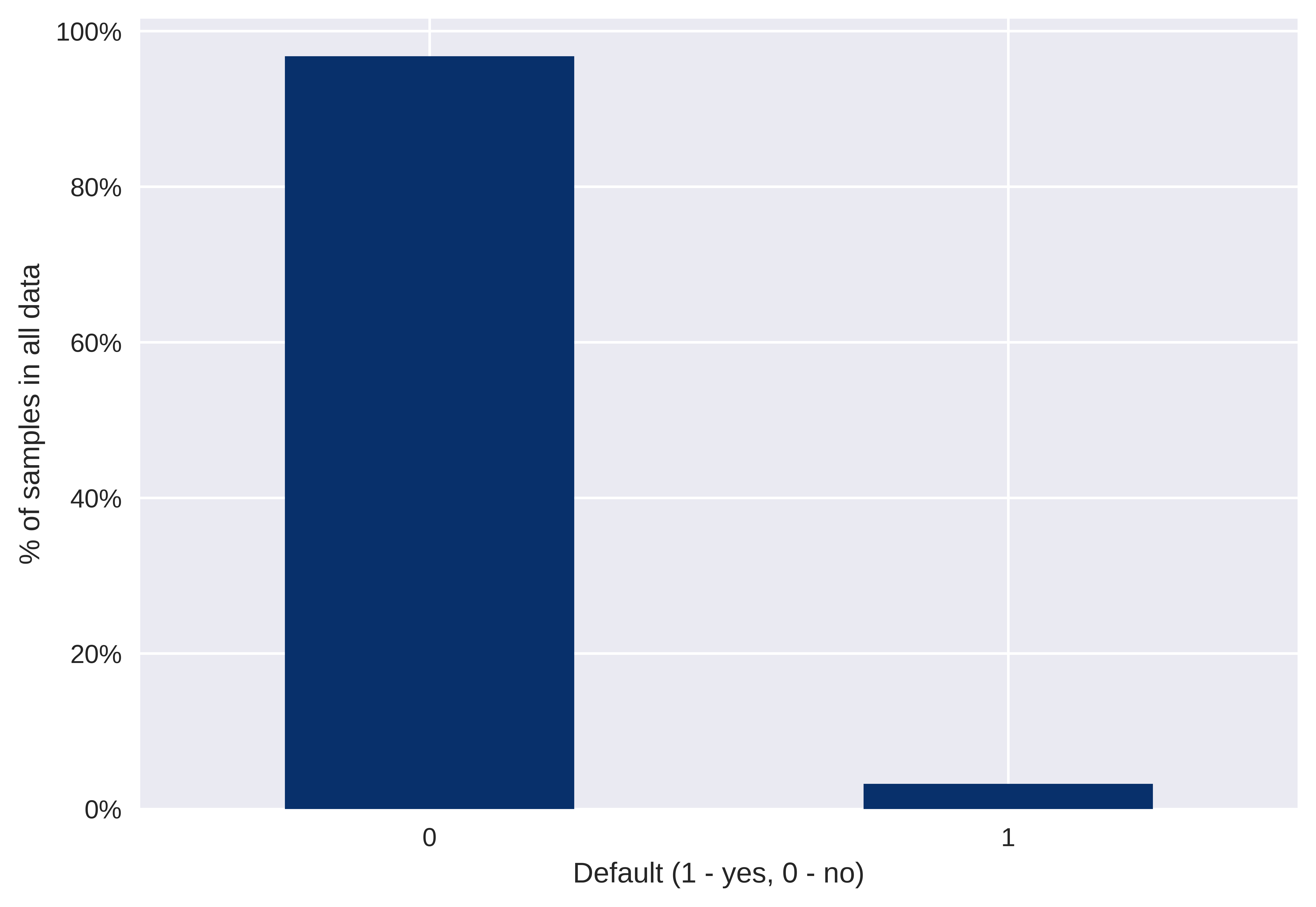
FIGURE 6.3: Imabalance in target variable.

Apart from the most straightforward features analysis, one of the crucial steps in our EDA was to verify the dependence between target variable and each of the features. We decided to use Kendall rank correlation coefficient, but we did not find any significant relationships between target and features (Figure 6.4).

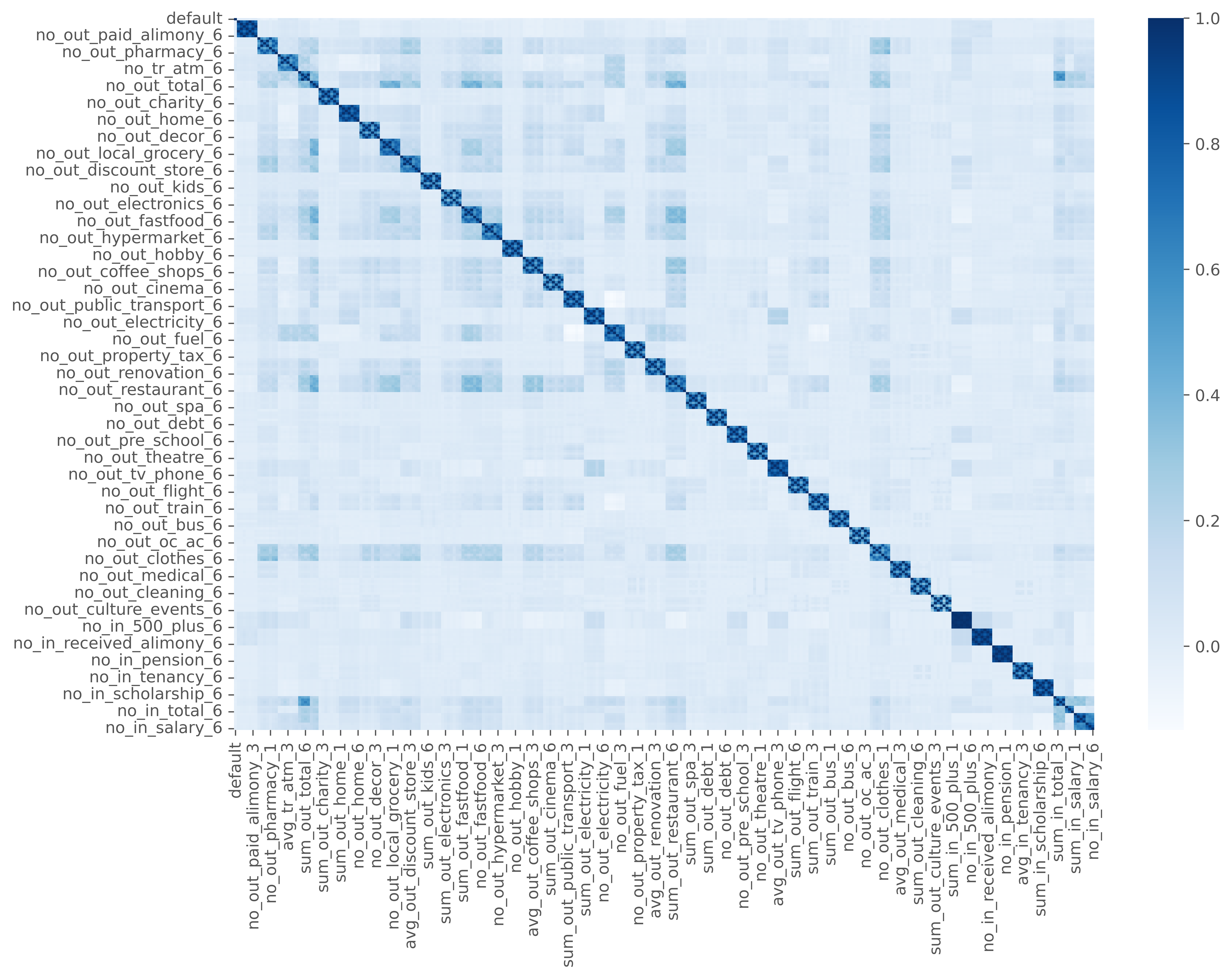
FIGURE 6.4: Pairwise Kendal rank correlation coefficient between features.

However, one approach that we’ve explored during EDA introduced us to an interesting conclusion that distribution of features for non-default clients usually has a longer tail than the distribution of the same feature for default ones. This could indicate that, based on some of the features, clients could be automatically classified as non-default ones if the value of the feature surpasses some threshold (Figure 6.5)

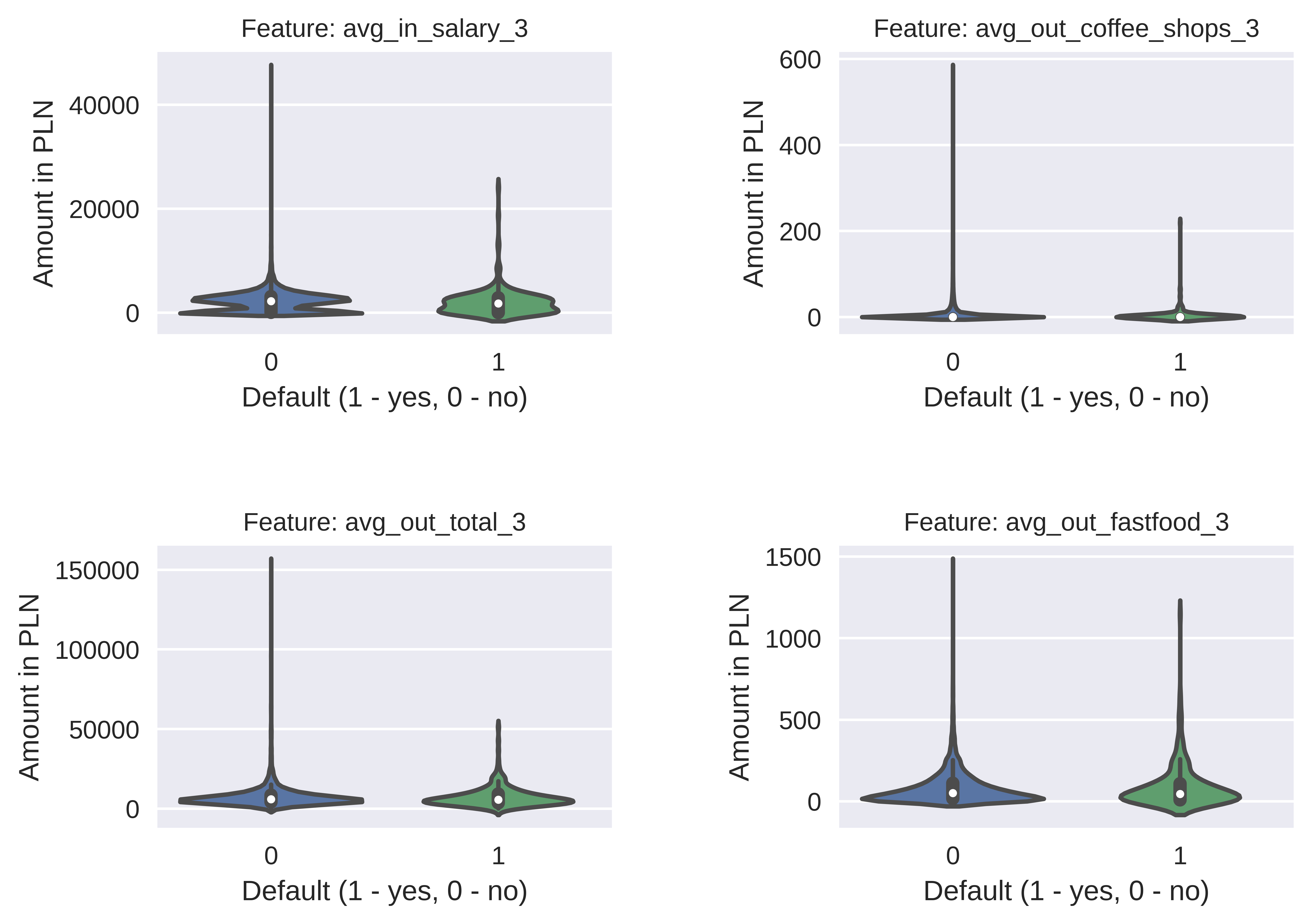
FIGURE 6.5: Example of features’ distributions.

6.3.2 Feature Engineering

Based on the results of the EDA and our initial research, we decided to engineer additional features to enrich our dataset. We’ve created them in the 4 following categories:

1. balance - this category represents difference between income and expenses in each of 3 given periods,
2. categories - we introduced additional 8 categories to aggregate similar expenses and we generated them for each of 3 periods (aggregated categories are show in Table 6.1),
3. periods - as our initial features were dependent on each other (for example expense from 1 month was a part of expenses in 3 months), we added independent periods of 6 to 4 months and 3 to 2 months based on the difference of features we had (see Figure 6.6),
4. proportions - one of our hypotheses from EDA was that default clients have a skewed proportion of certain categories in total expenses/incomes (eg. 90% of expenses is spent on restaurants) and hence we additionally calculated the proportion of each category on total income or expenses.

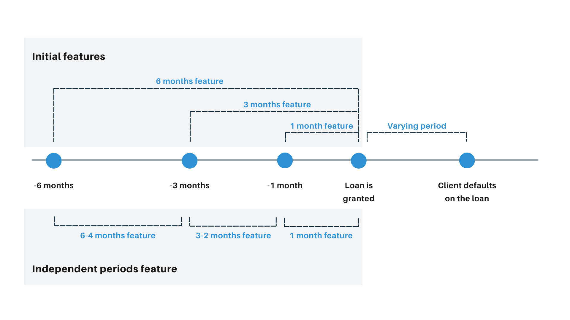
FIGURE 6.6: New monthly perspective used in periods features.

All of those 4 operations increased the number of usable features in our dataset to 762. More details on new naming convention and number of generated features can be found in Table 6.3.

TABLE 6.3: Features generated in the feature engineering process.

Type	Naming	Example	Number	Comment
Balance	balance_N	balance_1	3	N depends on the period, can be 1/3/6.
Categories	(category_name)_N	transport_6	24	N depends on the period, can be 1/3/6. Category names were shown in Data section.
Periods	(original_name)_NN	sum_out_decor_32	168	NN was the independent period, could be 64 or 32.
Proportions	(original_name)_propotion	sum_out_decor_1_proportion	273	-

6.4 Models and results

Due to the fact that data were in tabular form, but consisted of a large number of features, we decided to explore tree models and neural networks. Moreover, we also had to solve the problem of target variable imbalance. In order to do that, we additionally decided to explore the over- and under-sampling methods, as well as changing decision thresholds based on model output probability.

As there was no test data provided, we decided to use 5-fold cross-validation for testing purposes. In ordinary production setup, after obtaining average and per-fold scores we would train a single model on full dataset to use as final one, but since the problem was difficult (and hence - scores were low) and we had very restricted time, we decided to use a model from the best scoring fold as our final one.

Having the best interest of a bank on our mind, we decided to prioritise 2 business metrics to measure models’ results. Apart from that, we used 2 data science metrics for comparison. In all scores described in Table 6.4, the higher the value is, the better.

TABLE 6.4: Metrics used for model validation.

Metric	Type	Unit	Description
Average Profit	Business	PLN	Average profit the bank can earn from a single loan in a whole testing sample
Profit Ratio	Business	Percentage	Percentage of maximum profit the bank can earn from a single loan in a whole testing sample
Recall	Data Science	Percentage	Ratio of correctly predicted defaults to all defaults
F1	Data Science	Percentage	Harmonic mean of precision and recall

Below we present the final scores for our 2 best models: Random Forest and Multi-Layered Perceptron. Both used all the available features and 0.1 probability decision threshold. In the case of Random Forest, we used default sklearn hyperparameters, but we also added class balancing to overcome target class imbalance. In MLP, we similarly used default hyperparameters, but we additionally added data standardisation, minor class oversampling, as well as increased batch size to 2000 and increased L2 regularisation term to 0.001.

TABLE 6.5: Models’ final results.

Model	Average Profit	Profit Ratio	Recall	F1
MLP	334 PLN	69%	46%	27%
RF	330 PLN	68%	40%	29%

As we can see in Table 6.5, MLP obtained slightly better results in terms of average profit, profit ratio and recall. Both of them obtained significantly better results in terms of business metrics compared to random toss of a coin (Figure 6.7), which additionally shows that seemingly low data science scores can still produce valid and profitable business outcomes and automation potential.

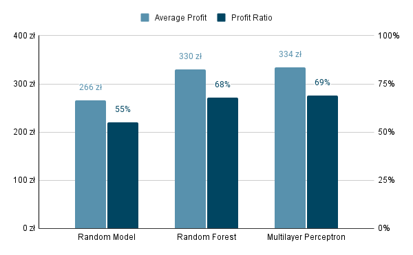
FIGURE 6.7: Comparison of the models to random model.

However, if we additionally take into account model stability with respect to probability decision threshold, we can see MLP raises more stable results which presents the potential for future optimization (Figure 6.8).

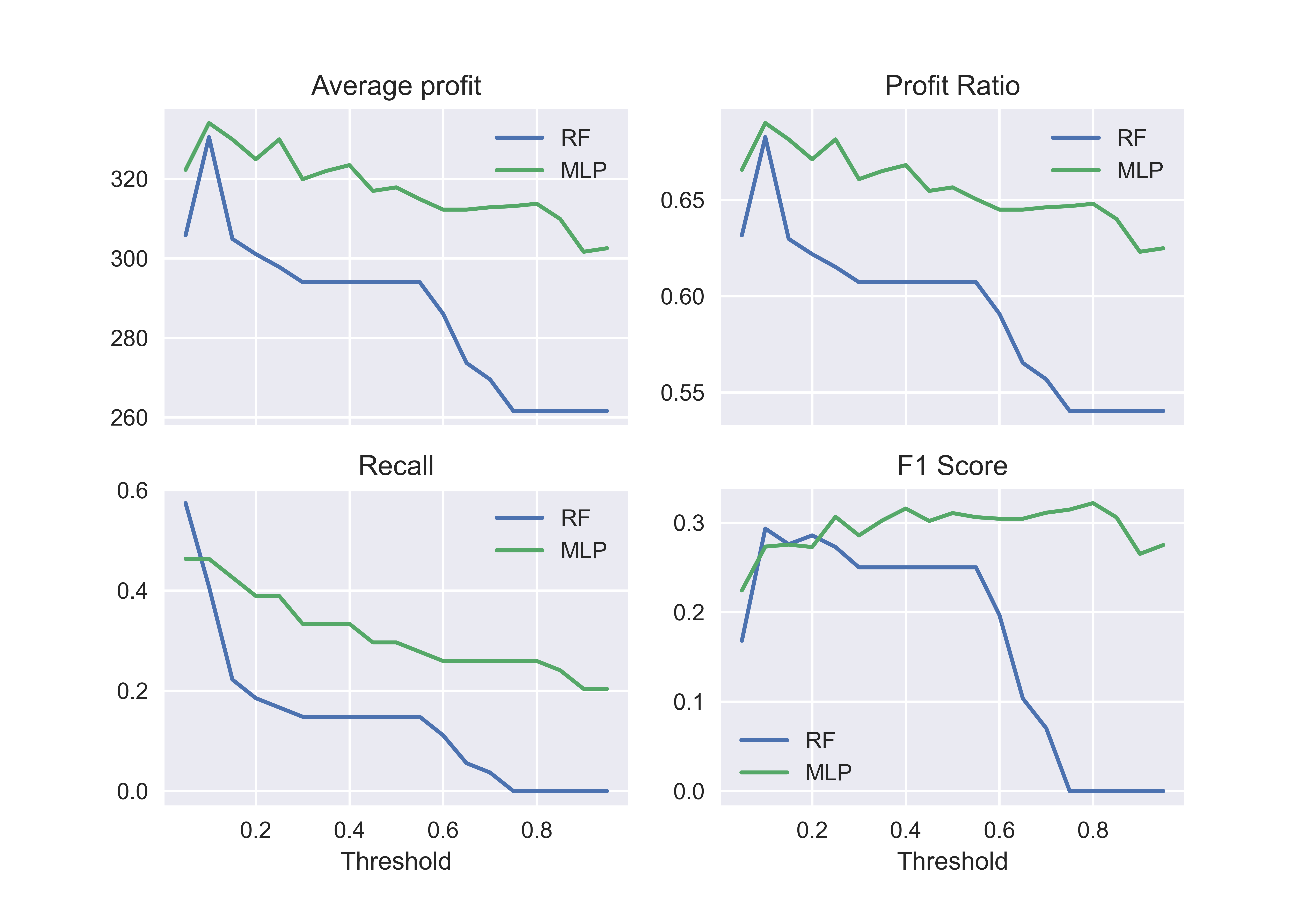
FIGURE 6.8: Metrics’ values with respect to decision threshold.

We additionally tried to solve the target class imbalance problem by filtering out low-risk clients from the dataset and assigning them non-default classes without running them through the ML model. For that, we wanted to use IF-ELSE statements based on our hypothesis from EDA that distributions of some features for non-default clients have long tails. We tried the approach in which for a given client if some feature surpassed a defined threshold, they were automatically a non-default one, so we could reduce the ratio of non-default to default clients in the training set for ML model. However, this approach drastically decreased our classifier’s scores.

We also tried hyperparameter tuning and feature selection for both models, but they too decreased our scores. In further parts of the report and the project, we decided to focus on the MLP model.

6.5 Explanations

Our approach to explanations was to:

• use Permutation Variable Importance (PVI) and Beeswarm SHAP plot to aggregate information used in the model from the whole dataset,
• create an intermediate step between global and local explanation using mixed Partial Dependence and Ceteris Paribus plots,
• move to local explanations using Shapley values to understand individual cases.

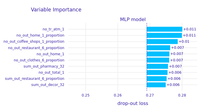
FIGURE 6.9: Permutation Variable Importance plot.

According to the PVI plot (Figure 6.9), we can observe that the number of ATM transactions and proportion of house expenses in all expenses had the largest contribution to models’ decision (both in favour and against giving a loan). Large number of proportion features in PVI plot also confirms our feature engineering hypothesis that proportion of specific expense or income category in all income and expenses may be a contributor to a client’s further loan-related decisions.

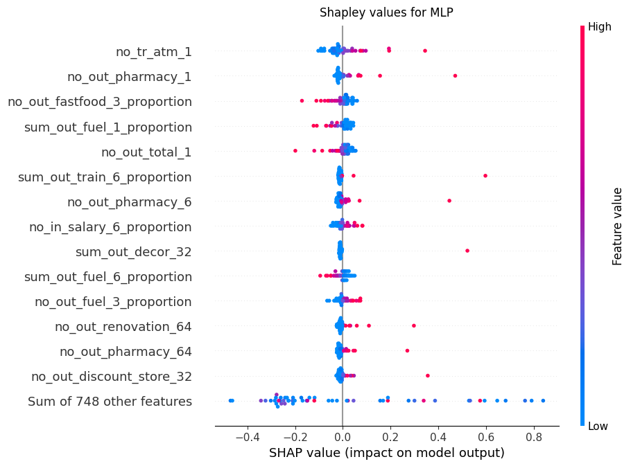
FIGURE 6.10: Shapley value beeswarm plot for default clients only.

The similar proportion tendency can be observed in SHAP beeswarm plot (Figure 6.10), which shows how specific feature values contribute to model output. We can observe that, on average, if the number of ATM transactions and pharmacy expenses becomes relatively high in a 1 month perspective, the contribution changes from negative to positive, meaning the client is more likely to be classified as default. On the other hand, we can also observe that fast-food or fuel proportion expenses have an inversely proportional relation. This means that higher values of those features are actually decreasing the chance of a client’s default.

Although those conclusions may seem unintuitive at first, we decided to think about the hypothesis on why such relations may occur. For fuel and fast-food expenses, we argue that if a client has proportionately high expenses in those categories, they also have a room for savings in case they have a problem in paying back the loan. Directly proportional relation with pharmacy expenses may be a result of the client’s increasing health problems, which could make paying back the loan less of a priority.

As the ATM and pharmacy expenses and their influence on the model interested us the most, we decided to gain a detailed perspective on them using PDP and CP plots.

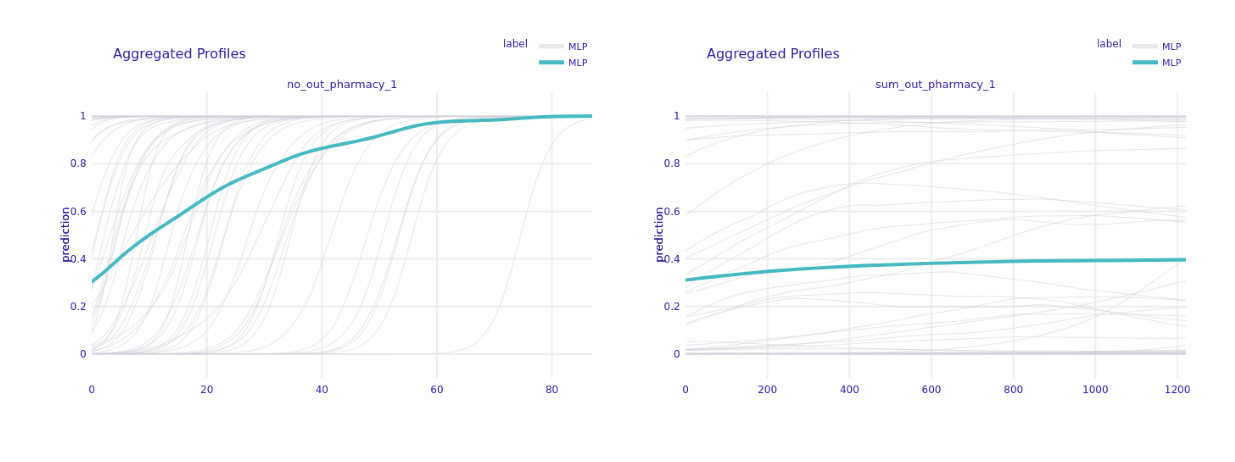
FIGURE 6.11: Partial Dependence Plot for sum and number of pharmacy transactions in 1 month period for default clients only.

As we can see in Figure 6.11, on average, increasing the number of pharmacy expenses in 1 month leads to a significant increase in the model’s output probability, which will lead to classifying clients as defaulting ones (green line). This tendency is also confirmed by individual, local CP plots (grey lines). However, when we look at the sum instead of the number of pharmacy expenses, this tendency is no longer as visible both in global and local aspects.

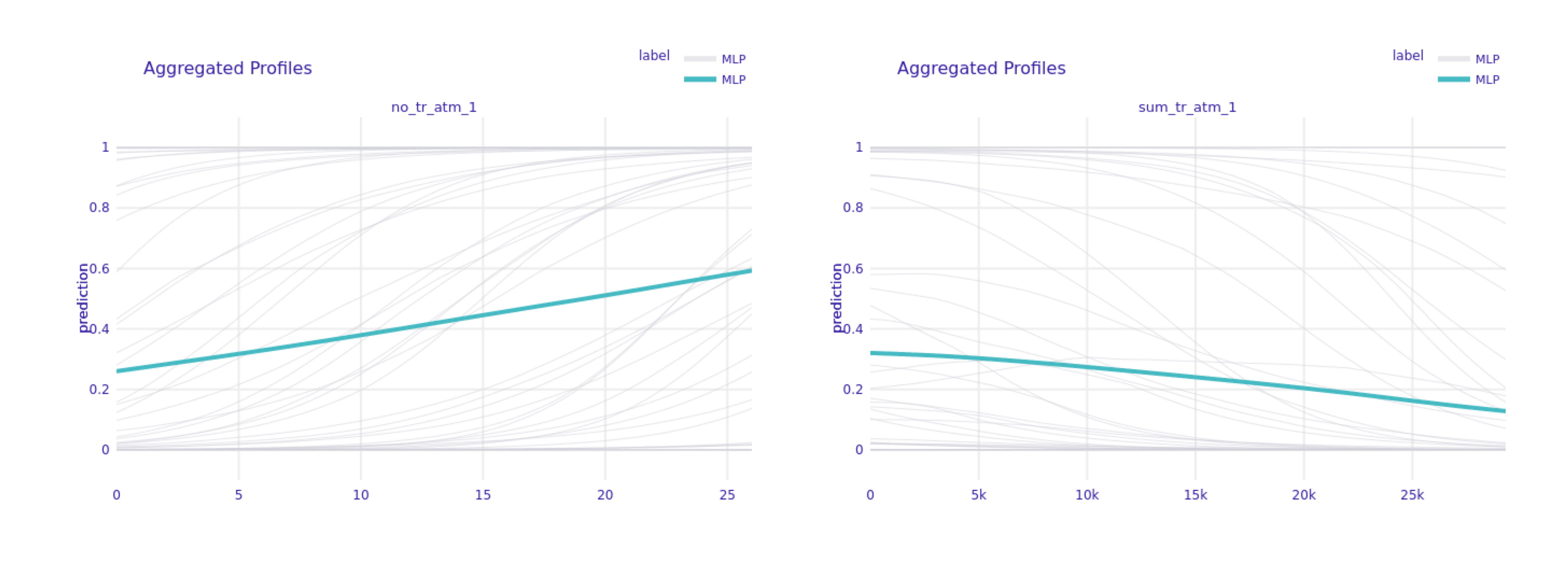
FIGURE 6.12: Partial Dependence Plot for sum and number of ATM transactions in 1 month period for default clients only.

Interestingly, the sum and number of ATM transactions in a 1 month perspective raise a completely different tendency in terms of the model’s decision (Figure 6.12). Whilst increasing number of transaction could indicate potential defaulting client (according to the model), the increasing total value of transactions would actually indicate otherwise.

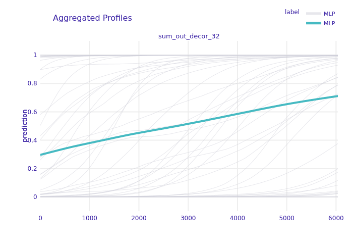
FIGURE 6.13: Partial Dependence Plot for total value of decor expenses between months 3 and 2 for default clients only.

There are also other features whose values have a directly proportional relation with the model’s probability, example of which is shown in Figure 6.13.

Last but not least, we decided to see if the features that highly contribute towards decisions in the local aspect are coherent with the image we obtained in a global one. We also wanted to put on the client’s hat for a moment and see how intuitive a given local explanation is.

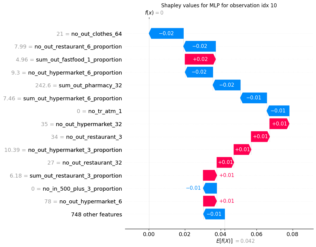
FIGURE 6.14: Shapley value for chosen correctly classified non-default example.

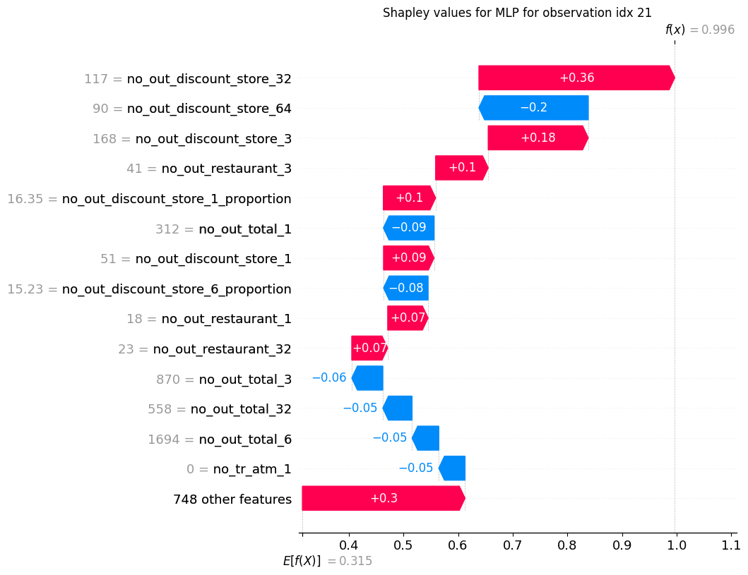
FIGURE 6.15: Shapley value for chosen correctly classified default example.

For both correctly predicted default (Figure 6.15) and non-default clients (Figure 6.14), we can see that on a local level we can actually focus on different features than the ones on which the model focuses on average globally. For an example default client, a really high contributor was the number of transactions in discount stores in different time perspectives before giving the loan, and for the non-default client - number of expenses on clothes.

Explanations, in our opinion, also show the potential limitations of our model. Finding out that a feature like pharmacy spending is a high decision contributor should lead to a close inspection with respect to fairness. Our hypothesis is that high pharmacy expenses may be a proxy for other features like client’s health or gender and therefore the model should not be used in production before this issue is checked, even if it provides higher than random profit from the loan.

6.6 User Study

In order to verify the usefulness of the model’s explanation process, we decided to create a survey to see if a potential bank’s client can distinguish between actual and random explanation with the increasing information overload.

6.6.1 Construction of the survey

The first part of the survey consisted of 4 questions to assess responders’ experience in the topic:

1. Have you ever studied in the field related to the financial market?
2. Have you ever worked in a position related to finance?
3. Have you ever applied for a loan?
4. Has your loan application been denied?

We also asked what, in their opinion, are the most important factors in decreasing a client’s chance of getting a loan.

Next, each responder was presented with 5 questions, each constructed in the same way.

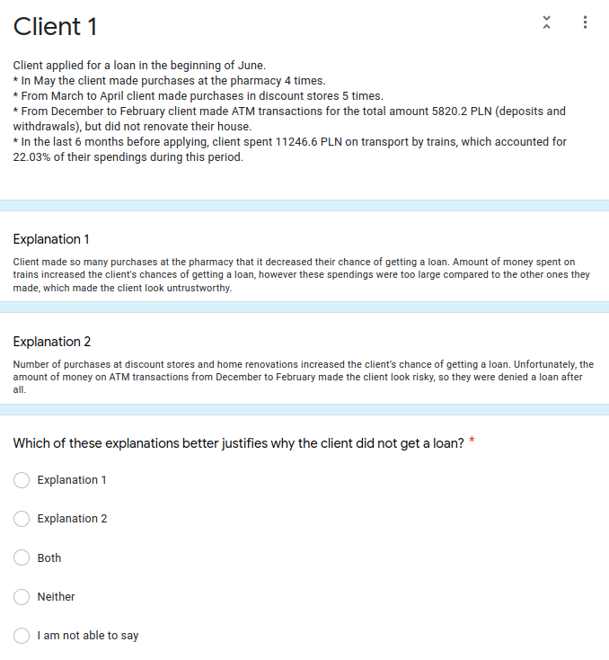
FIGURE 6.16: Example question from the survey.

Firstly, we provided the responder with a profile of a client who was denied a loan. In the profile, we used only the features which were later mentioned in the explanations.

Next, we gave the example of 2 explanations. One was generated using Shapley values for a chosen correctly classified default example from our dataset. The other was random and was constructed in the following way:

1. we chose 30 most important variables according to global SHAP values and excluded those used in a correct explanation,
2. we randomly selected N features from this subset, where N was the same number of features that was used in correct one,
3. we randomly chose the feature dynamics to be presented to the responder (from “too low”/“too high”).

In all 5 questions we used a different number of features per explanation, ranging from 3 to 7 to represent information overload. The responder was not informed that 1 of the explanations in done randomly.

Last but not least, each responder was asked to choose which explanation in their opinion is better in justifying the loan denial. Each responder could choose one of the explanations, both or neither of them or deny the answer completely. The full question is presented in Figure 6.16.

Finally, after the last question, we additionally wanted to check if responder opinion about most important features changed so we asked again about 3 most important factors decreasing a client’s chance of getting a loan.

6.6.2 Survey’s result

20 responders took part in the survey. Majority of them did not have any prior experience with the finance field, as well as the process of obtaining the loan (Figure 6.17).

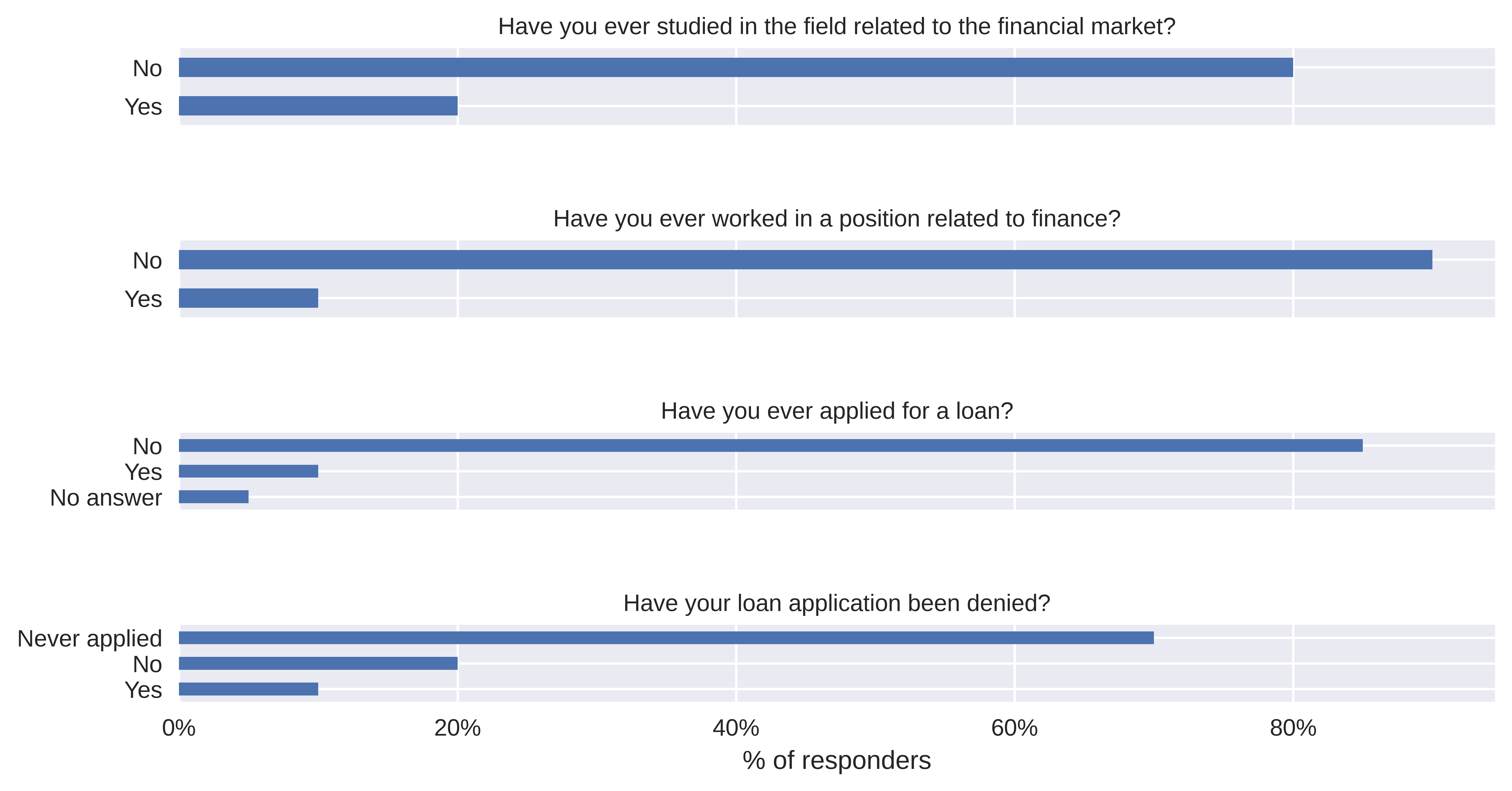
FIGURE 6.17: Summary of answers about experience in finance field and with taking a loan.

Before taking the survey, income was given as the number 1 perceived factor of potential loan denial, being mentioned by more than 90% responders (Figure 6.18).

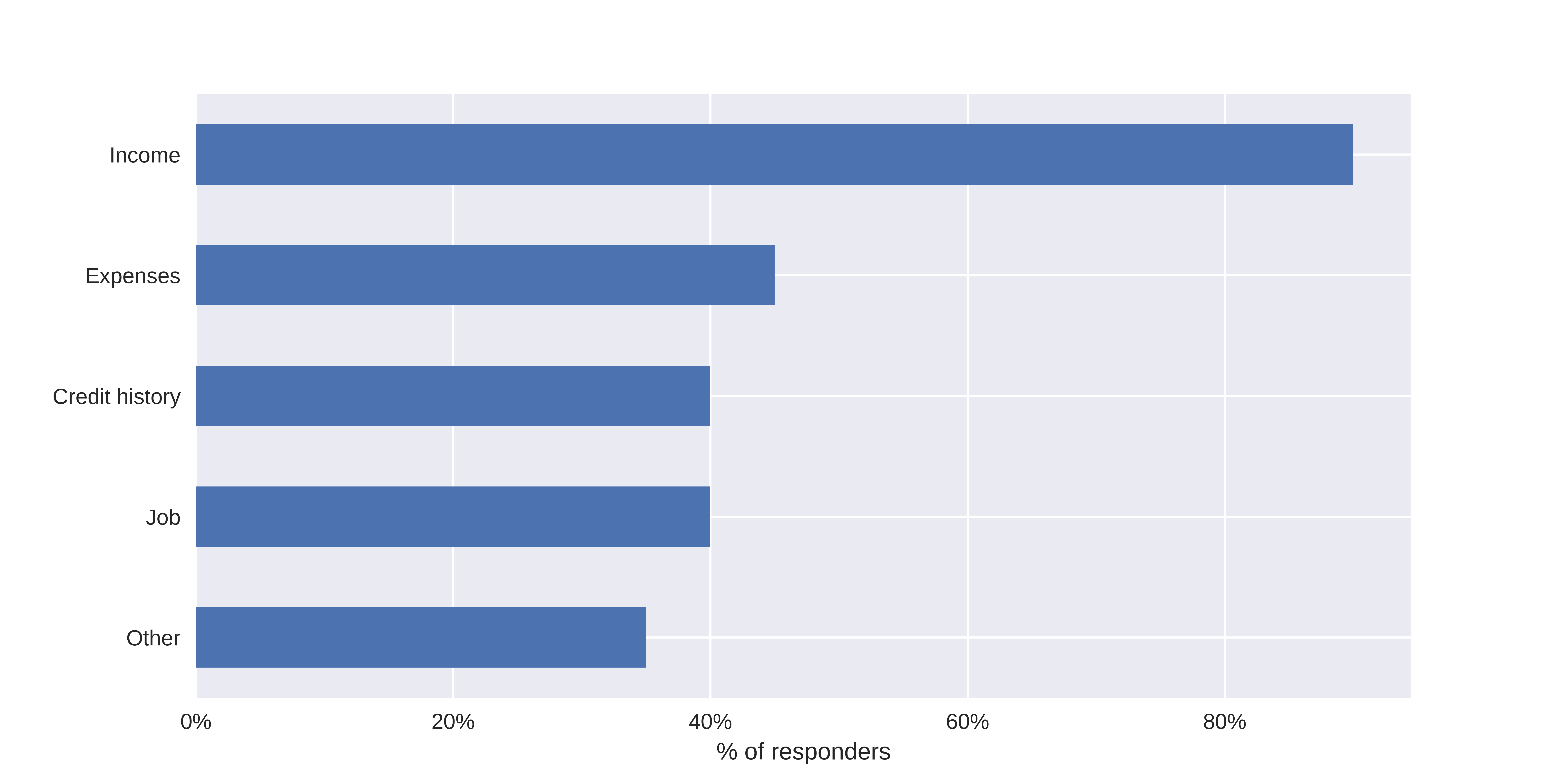
FIGURE 6.18: Factors chosen as most important in loan denial before taking a survey.

In Figure 6.19, apart from the outlying first question (with 3 explanations), there is some increasing tendency of giving a wrong answer once the number of information given also increases. However, the number of responders was too small to conclude it with high certainty.

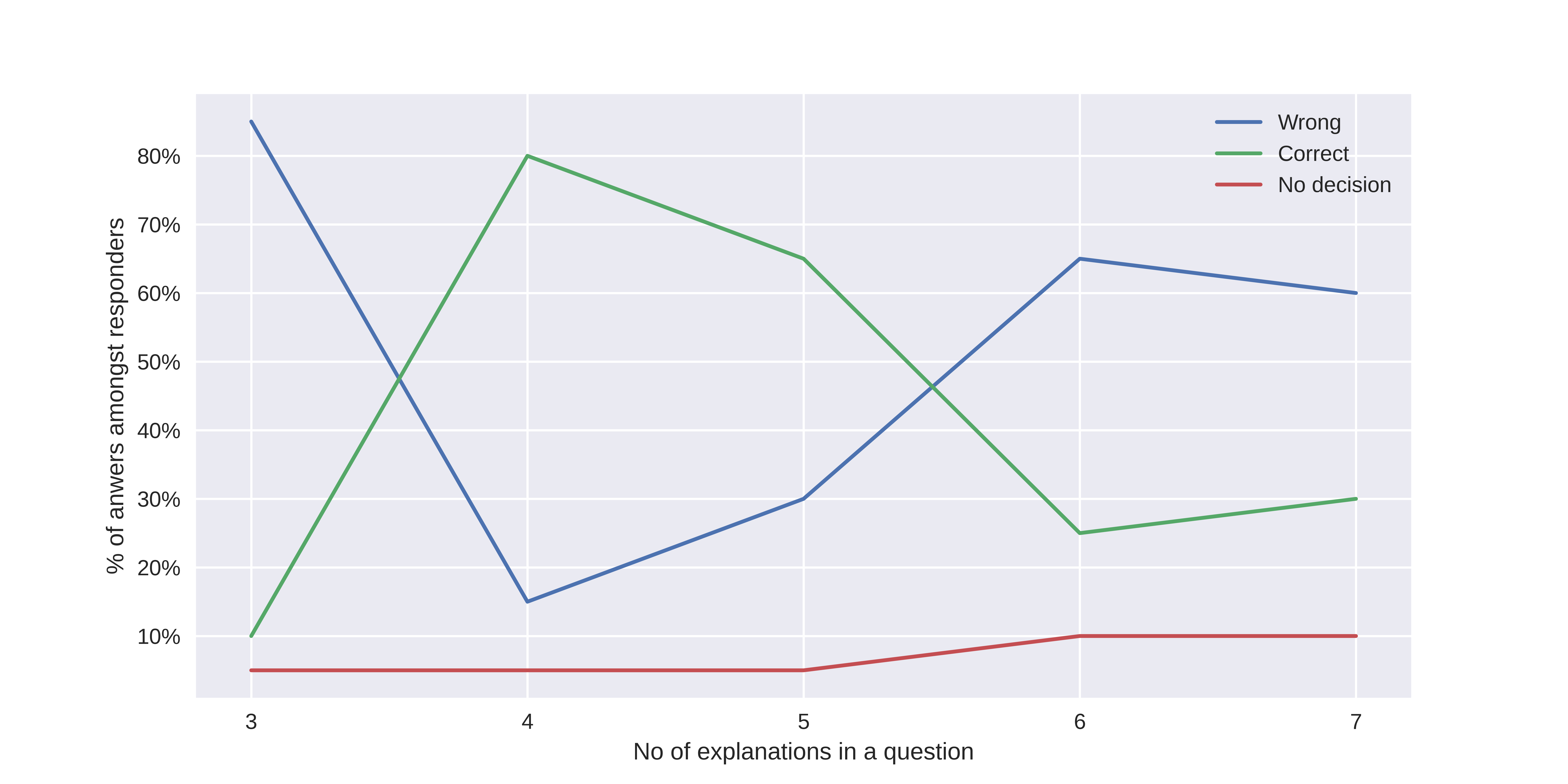
FIGURE 6.19: Answers quality with respect to number of information given.

Interestingly, after taking the survey, the dynamics of answering the question about critical denial factors changed. Expenses became the most frequent answer (more than 90% of responders) and the number of answers related to credit history or job significantly decreased (Figure 6.20).

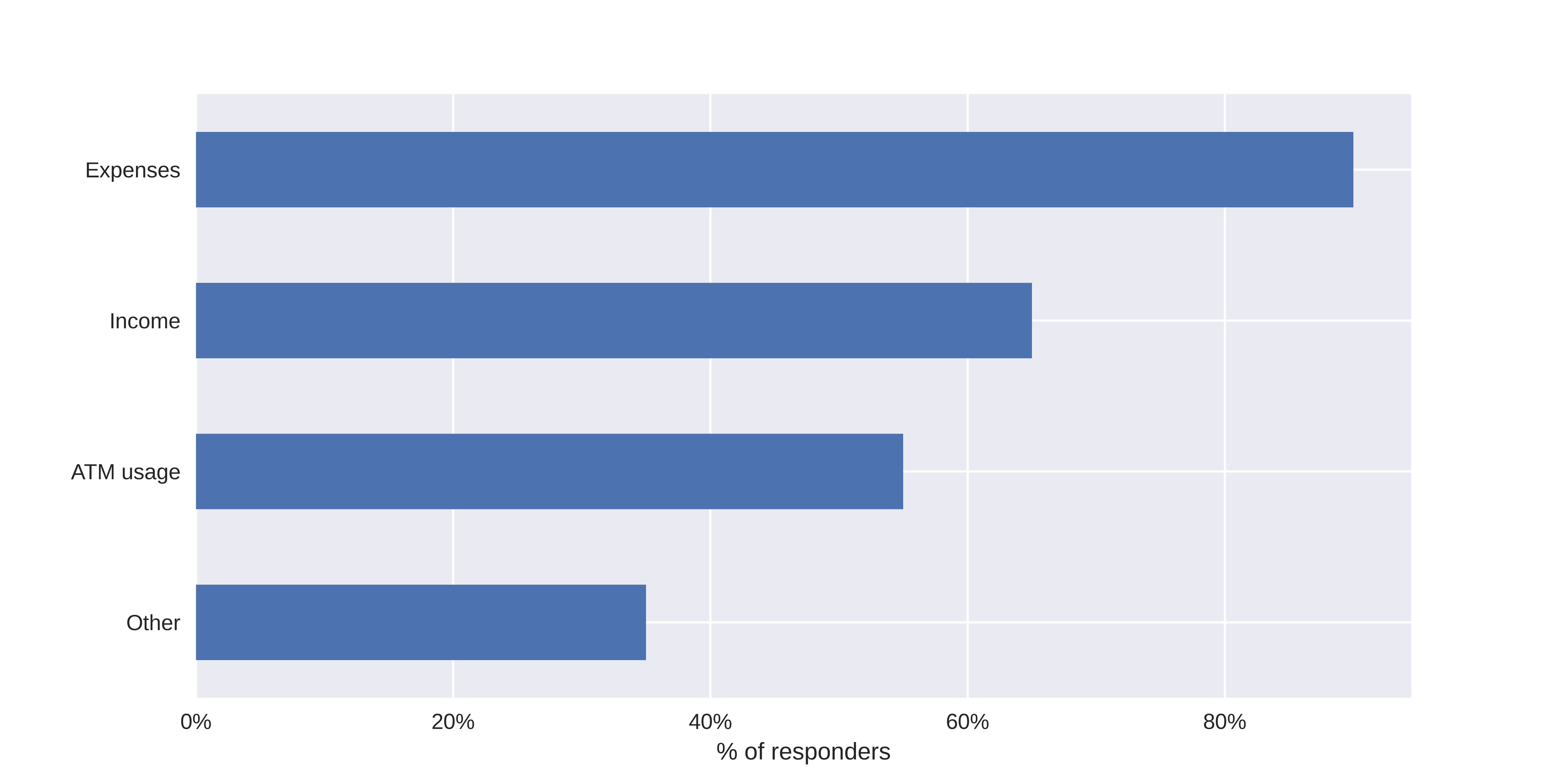
FIGURE 6.20: Factors chosen as most important in loan denial after taking a survey.

Moreover, specific expenses were now mentioned, similar to those used in the survey. This happened even though the question was not about the factors being taken into account by the model, but those that respondents feel were the most important in general (Figure 6.21).

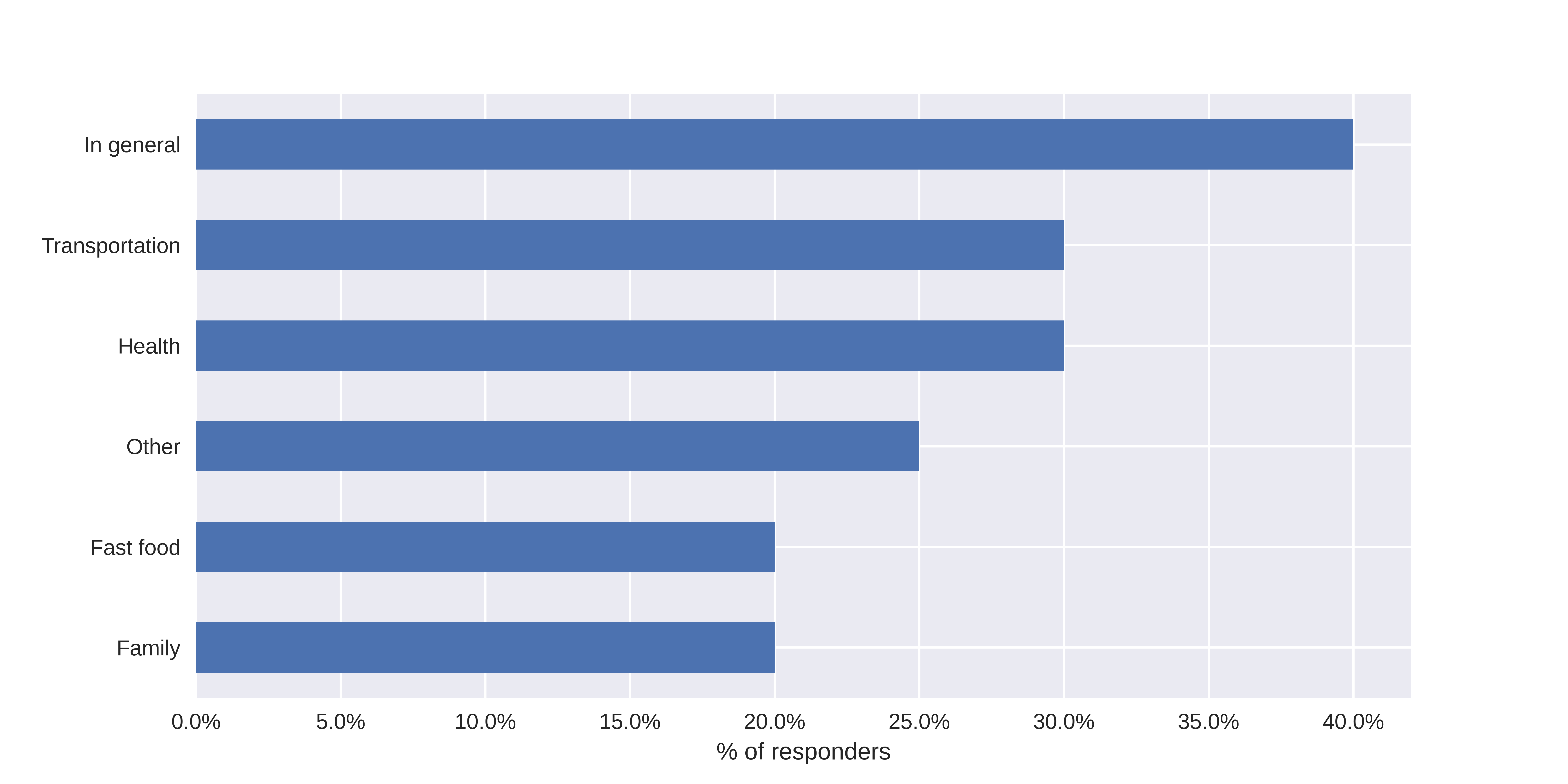
FIGURE 6.21: Expenses chosen as most important in loan denial after taking a survey.

This could hypothetically mean that when responders or clients are being exposed to many explanations, their view on general trends may change even though the explanations concern the model only (and hence - only approximations of the trend, and not necessarily correct ones). Such a hypothesis could be verified in another survey.

6.7 Summary

This report presented the results of a project in which we tried to verify the possibility of automating default prediction by a machine learning model. Default is the situation in which a client stops paying the loan back to the bank and is potentially harmful for the bank from the profit point of view. Our automation was done using clients’ expenses and incomes in 1 to 6 months perspective before being given a loan.

We managed to create 2 types of models, one of them being Multi-Layered Perceptron. We decided to use the bank’s average profit on a single loan as our model selection metric and we obtained an average profit of 334 PLN (69% of maximum profit).

An interesting observation that we produced during the model explanation phase was that it highly focuses on pharmacy expenses. Based on that, we hypothesise that, by proxy, our model may have problems with the fairness aspect (with respect to health and gender) and our recommendation would be to work on that aspect and increase the general model’s results in the future.

We also created a survey in which we wanted to verify if a potential bank’s client can distinguish between actual and random explanations with the increasing information overload. We observed that users prefer to see approximately 4 explanations on being denied a loan before they feel the information overload, but it should be confirmed on a larger and more diverse sample of clients.

Last but not least, the full code to the project will be available on GitHub after bank’s verification and approval.