Chapter 5 True income prediction based on client expenses
Authors: Dominik Kozłowski, Jakub Pietraszek, Kajetan Fornalik, Oliwia Skonieczka, Alan Drozd
Mentors: Marcin Bąk, Matteo Montoro
5.1 Introduction
The history of loans began thousands of years ago in Mesopotamia where the very first payday loans were used by farmers. Since then, the lending process evolved into a complex financial procedure. These days the banking industry is one of the most competitive which requires a constant need for development.
The development comes with a cost. Models that we use to predict the True income of clients become more and more complicated. The client may ask why? Why can’t you just add monthly salary, pension, rental income from properties, and other sources of income?
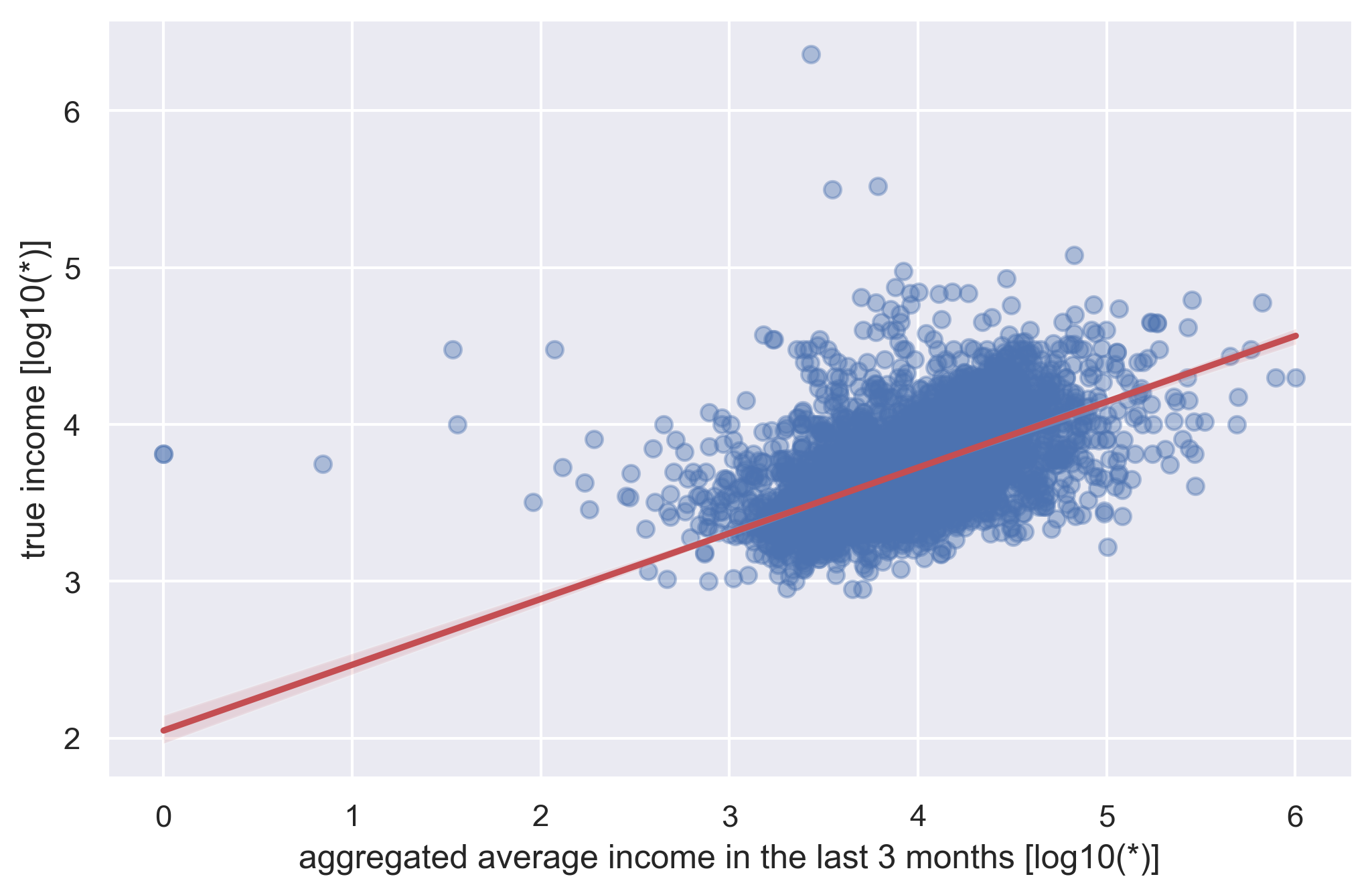
Deviation from true income
As you can see, if we try to predict the True income using just those few features we may end up with very inaccurate results. These kinds of mistakes may result in unnecessary losses for the bank. In order to improve True income prediction, we have decided to use more than 300 features related to client expenses in addition to those mentioned earlier to improve our results.
In this work, we want to find the model that is most accurate and easy to understand at the same time.
5.2 Dataset
We work on a dataset that was provided by mBank which is one of the biggest polish banks. The dataset consists of 20 000 rows, where each row corresponds to a different client.
Each client has 386 features that describe their revenue and spendings in the last 6 months (with granularity of 1 month/3 months/6 months). The predicted variable is the true income.
After initial analysis, we did not find any problems with the dataset, such as missing values or unusual values.
5.2.1 Groups
The variables were further divided into groups for later use in explainable methods.
| CATEGORY | FEATURE |
|---|---|
| SALARY | remuneration, pension |
| GENERAL INCOME | rent, scholarship, all other incomes |
| FOOD | grocery, deli shops, supermarkets |
| ATM | ATM |
| HOUSE | phone and TV subscription, electricity, rent, decors, electronics, cleaning services |
| CHILDREN | maintenance, toys, babysitter, camps, school |
| HEALTH | pharmacy |
| CAR | fuel |
| CULTURE | charity, hobby, events, theater, restaurants, clothes, fastfood, spa |
| FLIGHTS | flights |
| GENERAL OUTCOME | all other outcomes |
5.2.2 Preprocessing
Because the data are relatively clean, the only transformation performed was the logarithmization of the predictor variable.
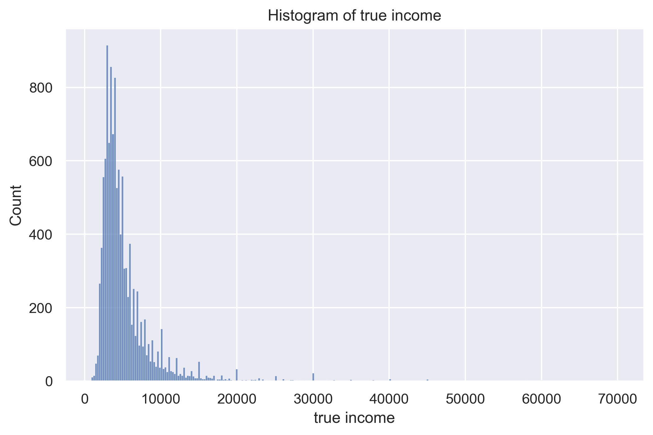
True income histogram
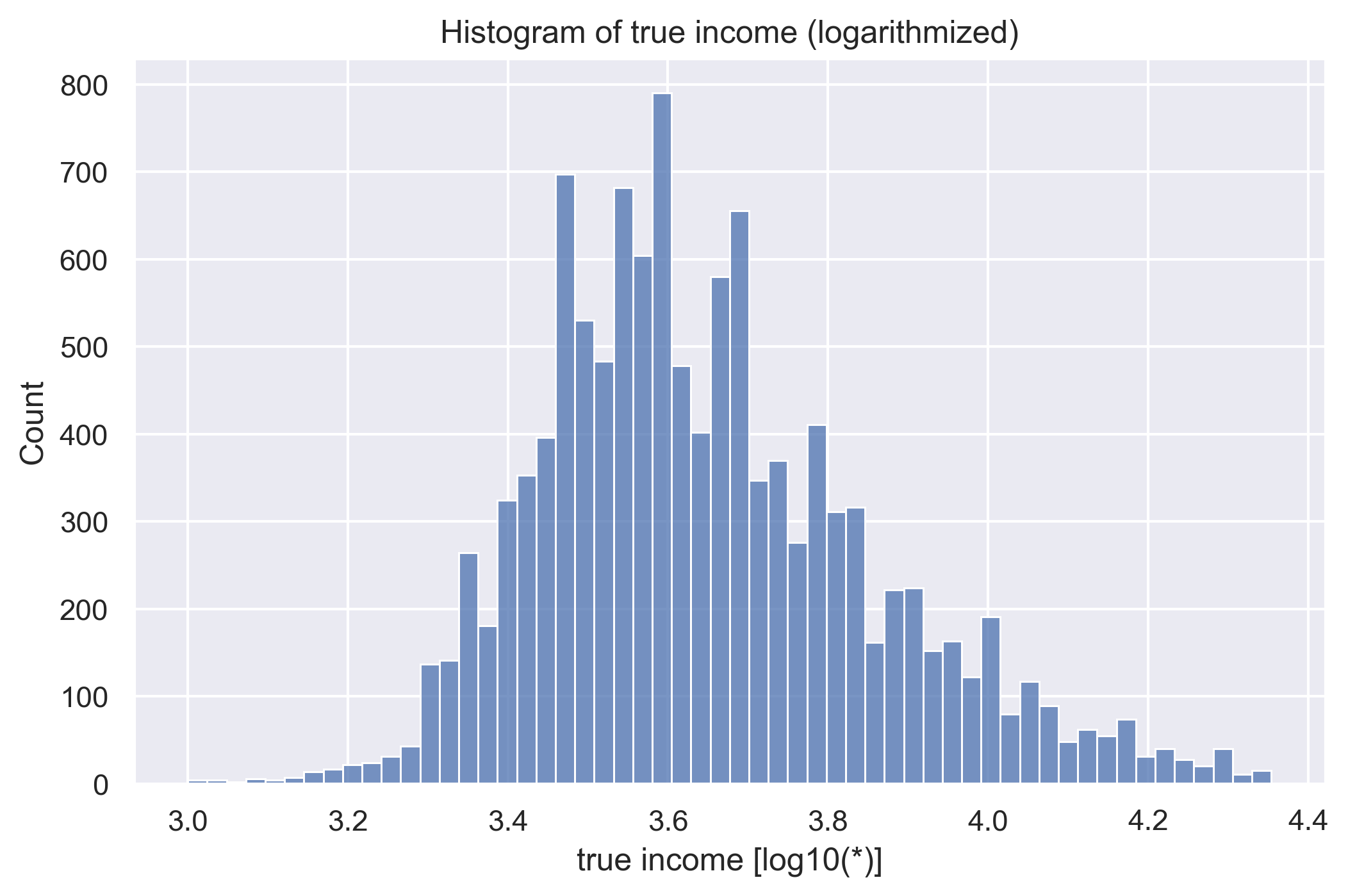
True income histogram
We have tried many preprocessing methods such as logarithmizations of the variables used for prediction or Winsorizing. Winsorizing is a method that sets all outliers to a specified percentile of the data. For example, a 98% winsorization would see all data below the 1th percentile set to the 1th percentile, and data above the 99th percentile set to the 99th percentile. Unfortunately, any gain in metrics was not statistically significant.
Normalization has not been performed, as the model, which we will mainly use, does not require it.
5.3 Models
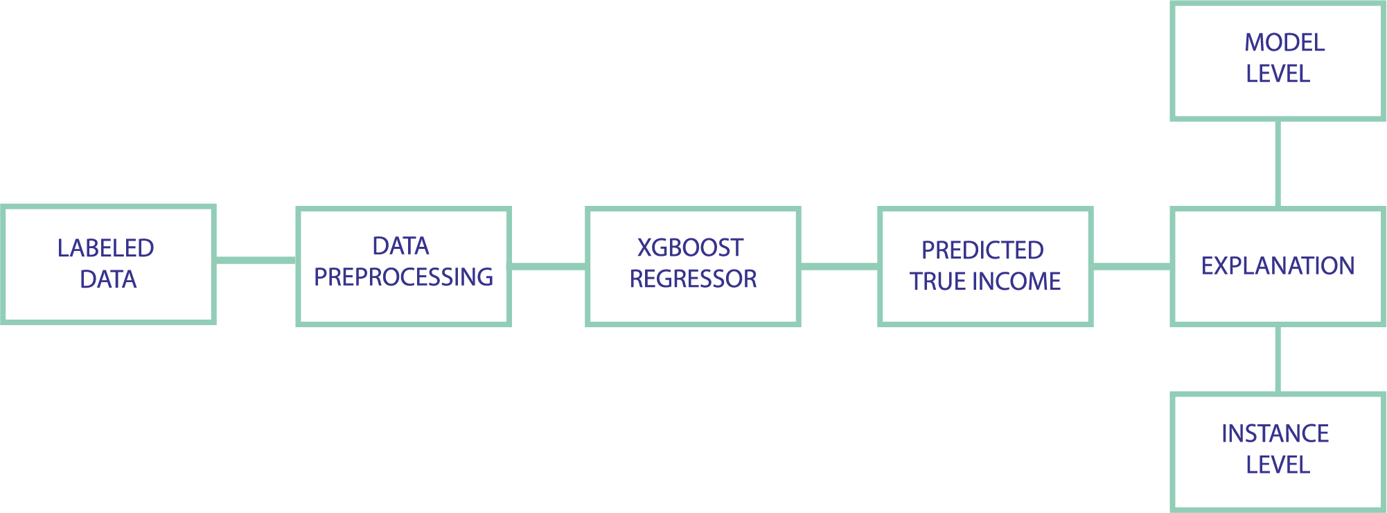
Pipeline of proposed model
5.3.1 Models description
As the data is in tabular form, our main model used to predict clients’ income was XGBoost, which has become the go-to solution for working on tabularized data. Additionally, in order to assess whether such a complicated model is required, we compare its performance with two other simpler models.
In summary:
- Dummy (always predicts median)
- Linear Regression (based on combinations of four features: age, job income, aggregated income, and spendings; in the last 6 months)
- XGBoost
5.3.2 Business metrics description
WPE-X
Measures what percentage of the predictions of the income falls into +-X% of its true value.
For example for the WPE-10, if the true income is 1000 PLN, then a prediction of 1050 PLN is within the range, but 700 PLN is not.
Concordance
The percentage of properly ordered pairs.
By proper order we mean that if true_income_1 < true_income_2 then pred_income_1 < pred_income_2 (resp. for the other way).
5.3.3 Model performance validation methodology
The dataset is splitted into 3 subsets (train-60% / validation-20% / test-20%) with stratification based on the predicted variable (income).
Optuna library is used for automatic hyperparameter optimization (if any). After the best parameters are found, we refit the model on the combined train and validation set and evaluate it on the test set.
5.3.4 Results
| model | val score (MAE) | test score (MAE) |
|---|---|---|
| Dummy | 2299.50 | 2388.32 |
| Linear Regression | 1870.96 | 1876.54 |
| Linear Regression (+true income logarithmization) | 1798.76 | 1866.84 |
| XGBoost | 2247.65 | 2808.47 |
| XGBoost (+true income logarithmization) | 1432.01 | 1445.02 |
| XGBoost (+true income logarithmization + parameters optimization) | 1325.21 | 1363.22 |
The XGBoost model significantly outperformed the simpler ones, yet only after logarithmization of the predicted variable.
Now we will evaluate it on the set of our metrics for business applications (income brackets are calculated on the entire dataset, by taking quantiles).
| business metric | Low Income | Low-Medium Income | Medium-High Income | High Income | All data |
|---|---|---|---|---|---|
| WPE-10 | 38.34% | 50.85% | 45.51% | 32.54% | 41.8% |
| WPE-20 | 59.56% | 75.62% | 73.06% | 51.74% | 64.98% |
| Concordance | 61.94% | 59.15% | 60.81% | 71.25% | 82.08% |
We see that the peak of performance is achieved in low-medium and medium-high income brackets, and there is a problem with low/high income. Concordance is almost the same across the subsets, yet it is higher in high income brackets, probably because of the lack of an upper bound.
To further assess the model’s performance and its characteristics, we may look into its residuals
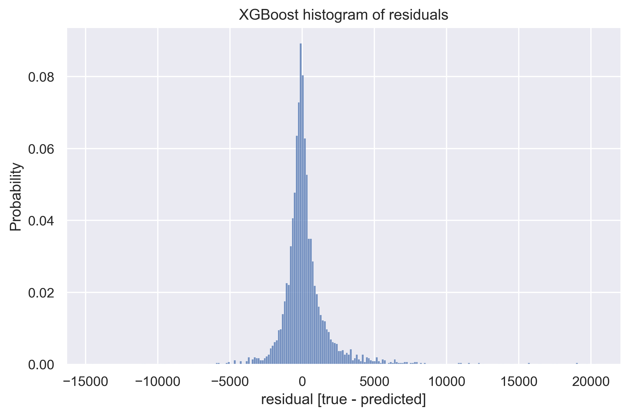
XGbBoost residuals - histogram
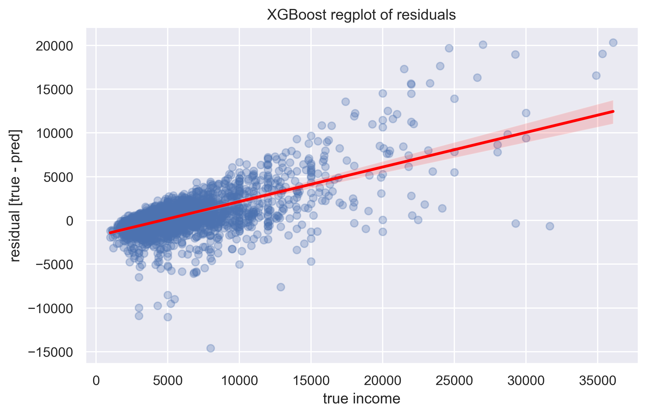
XGbBoost residuals - regplot
By looking at the second plot, particularly at its linear regression line (red color). We can state that the problem in low income bracket is overestimating clients’ income, and in high income bracket, underestimating it. Incorporating this knowledge into the model (by for example manually changing its predictions, by some constant, in low/high income brackets) would require more elaborated validation methodology so we left it as a possible further improvement.
Now we will plot capture rate.
The algorithm to compute it is as follows:
- take some threshold value T
- subset all samples where true income is bigger than T
- make predictions on these samples
- calculate the ratio of predictions that fall over the threshold T with respect to the total size of the subset
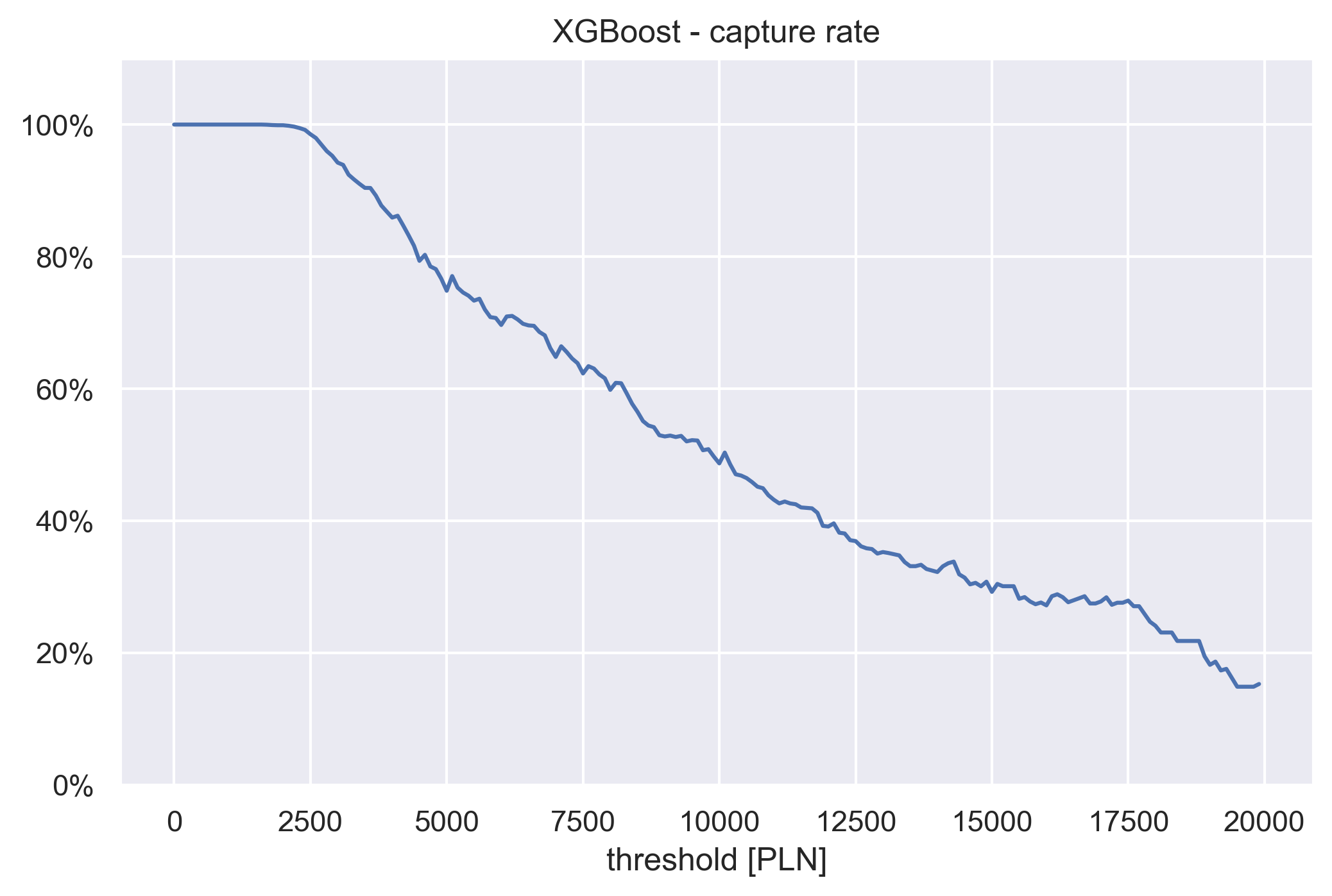
XGbBoost capture rate
If we take a threshold value of 5000 PLN, we can read from the plot that if the true income of our client is over 5000 PLN, then there is ~77% chance that our prediction is also over 5000 PLN. Such information could be of use during estimation of credit risk.
Also, we can transform the problem from regression to a classification one, by picking some threshold value, and setting all the income below it to 0 and above it to 1.
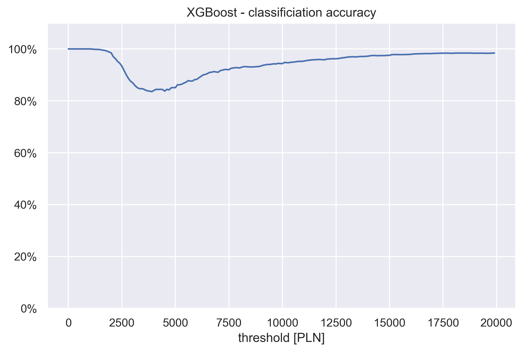
XGbBoost classification accuracy
By plotting the classification accuracy over different thresholds, we obtain a view of the capture rate that also takes into account the directionality.
5.4 Explanations
Here we present our methods for making our project explainable. We have used instance level and model level tools. All of it was done with dalex library in Python.
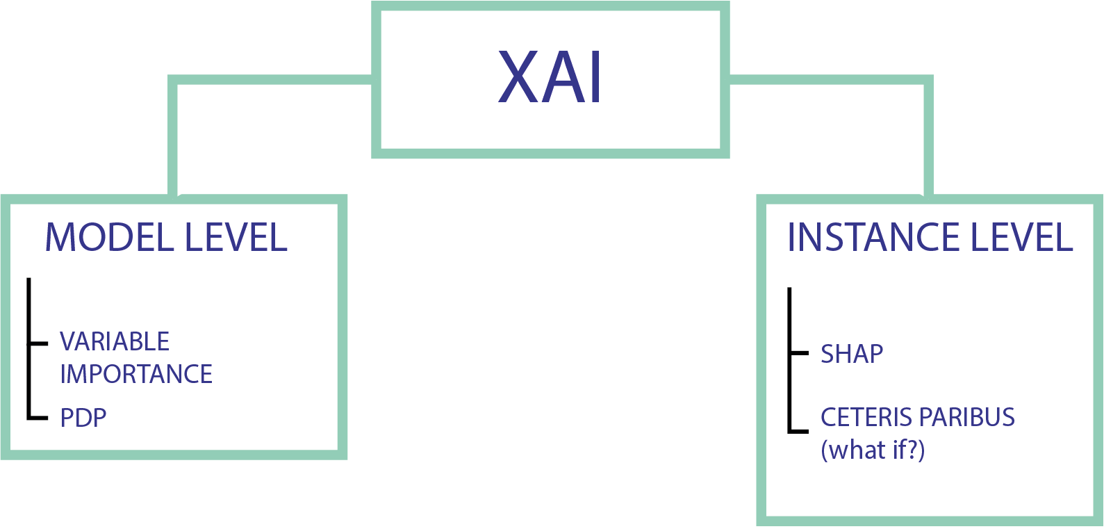
Explanations pipeline
5.4.1 Model level
5.4.1.1 Variable Importance
One of the essentials in XAI is understanding which predictor variables are relatively influential on the predicted outcome.
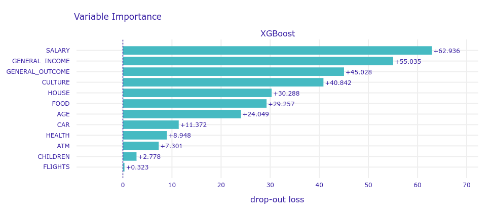
As you can see above, variable importance to a certain extent overlaps with intuition. The most important group of variables is salary, then general income, outcome, and expenses for culture (theater, restaurants, SPA, etc). Expenses for car, health, children and flights are rather insignificant.
5.4.1.2 PDP
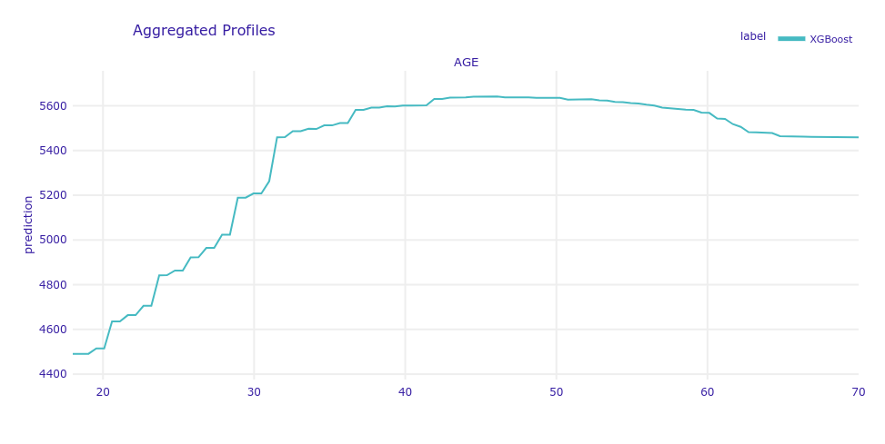
The model profile function calculates explanations on a dataset level set that explore model response as a function of selected variables.
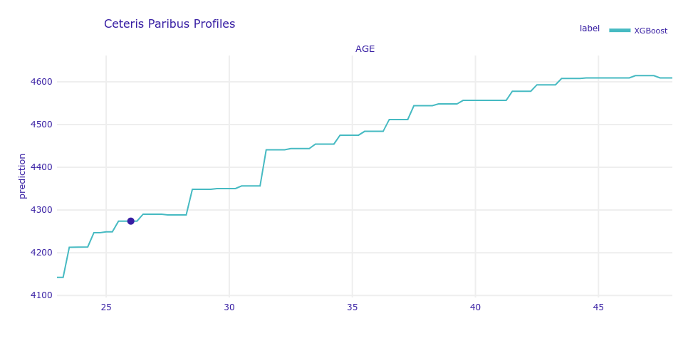
Below you can see the Partial Dependencies Profile for the age variable. Despite its relatively low importance for the model, this variable has one of the most interesting profile in the dataset, as it is not linear. The same we could find in SHAP, age has a big impact on prediction for young people.
5.4.2 Instance level
5.4.2.1 SHAP
SHapley Additive exPlanations is a game theoretic approach to explain the output of any machine learning model. It connects optimal credit allocation with local explanations using the classic Shapley values from game theory and their related extensions.
Below you can see SHAP chart for one of the predictions. To simplify explainability, we sum Shapley values into previously established groups of incomes and outcomes.
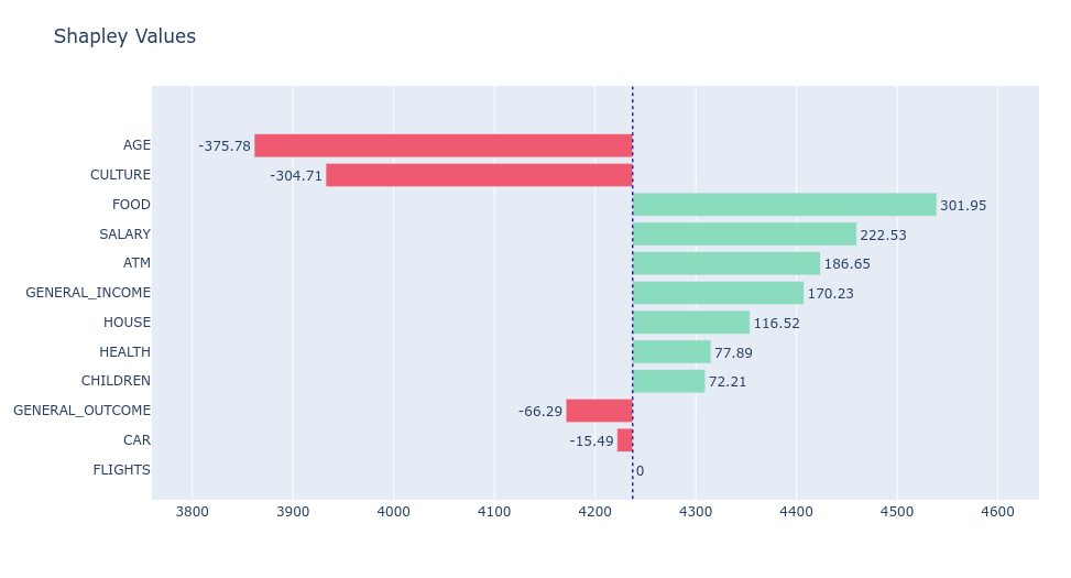 Due to the conclusion in previous methods, variable groups like flights, cars, and children have rather a small impact on prediction. The biggest impact on model prediction has the age variable, which was not in the first positions of the variables’ importance plot. Ceteris Paribus Profile is a great tool to explain this for this case. As previously mentioned, age is not linear in this case, and causes a much lower model prediction.
5.5 Usage and user experience
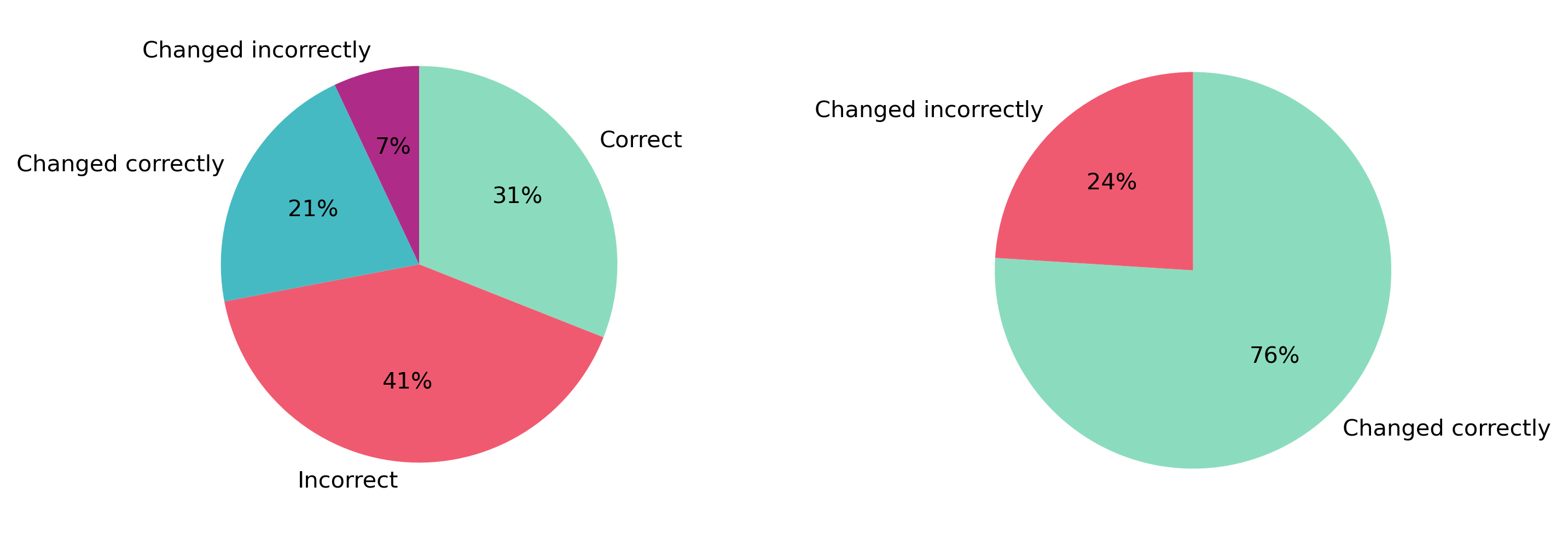
Our model has two main usages. The first is that it helps a bank to predict the true income of their potential client since more often than not it’s hard to estimate this value only based on information that client provides. The second application of our model is to help explain a bank’s decision to a client. It’s important that the client understands what influences the final verdict, which in return reinforces his confidence in both the bank and the model. To examine the explainability of our model, we created a questionnaire in which we compared guesses based on intuition (on raw data) and guesses based on model prediction. It was sent over to a number of subjects of different ages, genders, occupations, and education levels.
For questionnaire purposes, we divided income values into 3 sets based on quantiles of our full data. People with low income (below 1/3 quantile), people with average income (up to 2/3 quantile) and people with high income (anything above 2/3 quantile). In questionnaire, readers were tasked to predict the income level of 9 random people. For each person, they firstly made a prediction based on values of general income, general expenses, remuneration, and cultural expenditure (four most important variables in the model). After the first question, they were presented with our model’s SHAP break-down, based on which they could alter their initial guess.
5.5.1 Results
From those questionnaires, we got the following results. Firstly, we were happy to see that the model was performing much better than “human intuition”. Initial guesses were wrong 68.9% of the time, which implies the need for other tools, like our model. Secondly, 76% of people who changed their initial prediction after seeing the model’s explanation, corrected their guess. That tells us that with a little more explaining, there shouldn’t be any trouble for bank’s clients to understand the model’s explanation. Lastly, there was a glaring problem with how many people have chosen incorrect answers. After talking to some people who took the questionnaire, it turned out that some parts were written unclearly to them, with words like quantile e.t.c.
This strongly impacted negatively on the questionnaire’s results. With more time it would be worth it to simplify the questionnaire and run it again.
5.6 Summary
In this report, you can see the results of our combined efforts in predicting income using machine learning methods. We aimed to achieve a model which is both reliable in making predictions and easy to understand by the average person.
The survey we created shows us that it is important to talk in straightforward words to clients for a better understanding of XAI methods, without complicating it by overloading mathematical vocabulary.
To sum up, from the beginning we aimed to create an explainable model, as even the best model which we do not know exactly how it works is useless for business purposes.
We believe that after many attempts, we managed to create a model, which was able to predict client true income with satisfying accuracy without losing its explainability. The metrics we show were aimed to be as much as possible explainable for business receivers.